
Configuring Simulator object
The following code is used to produce the figures in this section.
>>> import matplotlib.pyplot as plt
>>> import matplotlib as mpl
>>> mpl.rcParams["figure.figsize"] = (6, 3.5)
>>> mpl.rcParams["font.size"] = 11
...
>>> # function to render figures.
>>> def plot(csdm_object):
...     # set matplotlib axes projection='csdm' to directly plot CSDM objects.
...     ax = plt.subplot(projection='csdm')
...     ax.plot(csdm_object, linewidth=1.5)
...     ax.invert_xaxis()
...     plt.tight_layout()
...     plt.show()
Up until now, we have been using the simulator object with the default setting.
In mrsimulator, we choose the default settings such that it applies to a wide
range of simulations including, static, magic angle spinning (MAS), and
variable angle spinning (VAS) spectra. In certain situations, however, the
default settings are not sufficient to accurately represent the spectrum. In
such cases, the user is advised to modify these settings as required. In the
following section, we briefly describe the configuration settings.
The Simulator class is configured using the
config attribute. The default value
of the config attributes is as follows,
>>> from mrsimulator import Simulator, SpinSystem, Site
>>> from mrsimulator.methods import BlochDecaySpectrum
...
>>> sim = Simulator()
>>> sim.config
ConfigSimulator(number_of_sidebands=64, integration_volume='octant', integration_density=70, decompose_spectrum='none')
Here, the configurable attributes are number_of_sidebands,
integration_volume, integration_density, and decompose_spectrum.
Number of sidebands
The value of this attribute is the number of sidebands requested in evaluating the spectrum. The default value is 64 and is sufficient for most cases, as seen from our previous examples. In certain circumstances, especially when the anisotropy is large or the rotor spin frequency is low, 64 sidebands might not be sufficient. In such cases, the user will need to increase the value of this attribute as required. Conversely, 64 sidebands might be redundant for other problems, in which case the user may want to reduce the value of this attribute. Note, reducing the number of sidebands will significantly improve computation performance, which might save computation time when used in iterative algorithms, such as least-squares minimization.
The following is an example of when the number of sidebands is insufficient.
>>> sim = Simulator()
...
>>> # create a site with a large anisotropy, 100 ppm.
>>> Si29site = Site(isotope='29Si', shielding_symmetric={'zeta': 100, 'eta': 0.2})
...
>>> # create a method. Set a low rotor frequency, 200 Hz.
>>> method = BlochDecaySpectrum(
...     channels=['29Si'],
...     rotor_frequency=200, # in Hz.
...     spectral_dimensions=[dict(count=1024, spectral_width=25000)]
... )
...
>>> sim.spin_systems += [SpinSystem(sites=[Si29site])]
>>> sim.methods += [method]
...
>>> # simulate and plot
>>> sim.run()
>>> plot(sim.methods[0].simulation)


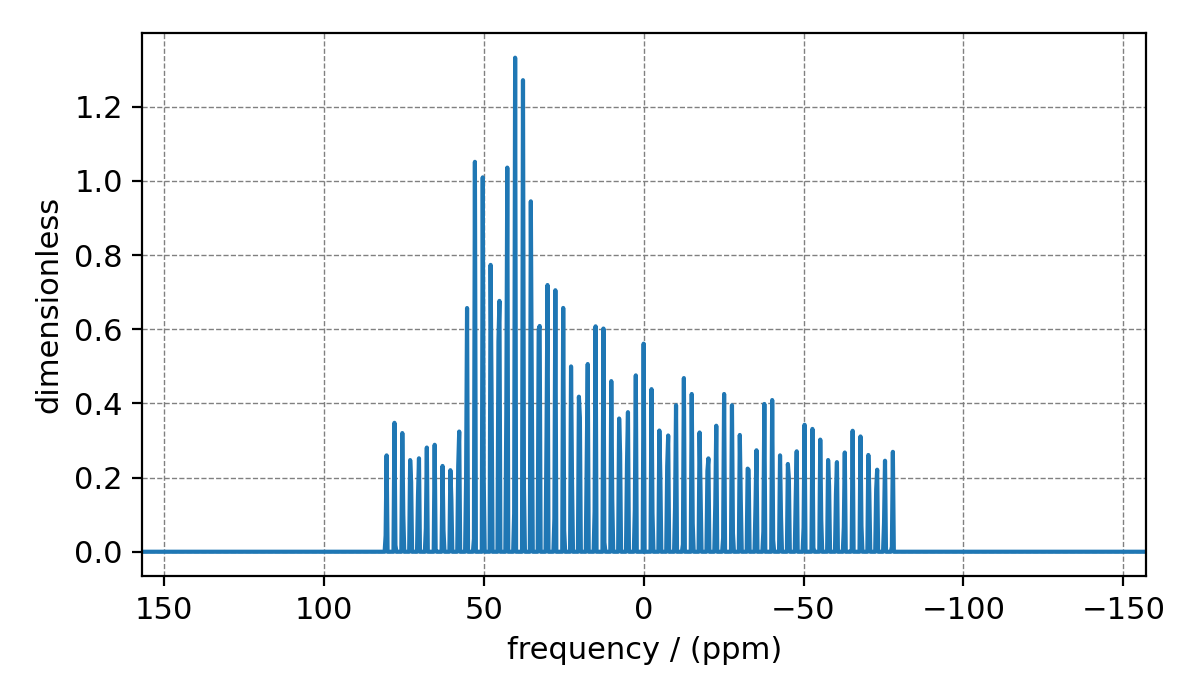
Figure 11 Inaccurate spinning sidebands simulation resulting from computing a relatively low number of sidebands.
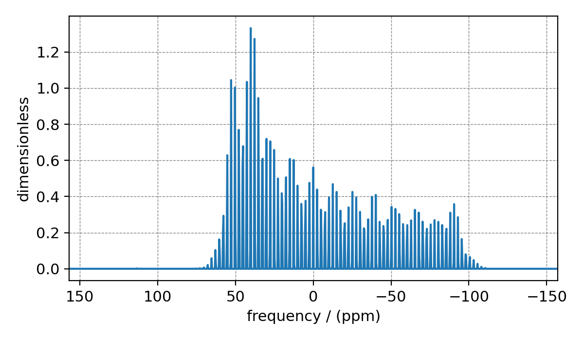
If you are familiar with the NMR spinning sideband patterns, you may notice that the sideband simulation spectrum in Figure 11 is inaccurate, as evident from the abrupt termination of the sideband amplitudes at the edges. As mentioned earlier, this inaccuracy arises from evaluating a small number of sidebands relative to the given anisotropy. Let’s increase the number of sidebands to 90 and observe. Figure 12 depicts an accurate spinning sideband simulation.
>>> # set the number of sidebands to 90.
>>> sim.config.number_of_sidebands = 90
>>> sim.run()
>>> plot(sim.methods[0].simulation)

Figure 12 Accurate spinning sideband simulation when using a large number of sidebands.
Integration volume
The attribute integration_volume is an enumeration with two literals, octant and
hemisphere.
The integration volume refers to the volume of the sphere over which the NMR frequencies
are integrated. The default value is octant, i.e., the spectrum comprises of integrated
frequencies arising from the positive octant of the sphere.
The mrsimulator package enables the user to exploit the orientational symmetry of
the problem, and thus optimize the simulation by performing a partial integration
—octant or hemisphere. To learn more about the orientational symmetries,
please refer to Eden et. al. 1
Consider the \(^{29}\text{Si}\) site, Si29site, from the previous example. This
site has a symmetric shielding tensor with zeta and eta as 100 ppm and 0.2,
respectively. With only zeta and eta, we can exploit the symmetry of the problem,
and evaluate the frequency integral over the octant, which is equivalent to the
integration over the sphere. By adding the Euler angles to this tensor, we break the
symmetry, and the integration over the octant is no longer accurate.
Consider the following examples.
>>> # add Euler angles to the shielding tensor.
>>> Si29site.shielding_symmetric.alpha = 1.563 # in rad
>>> Si29site.shielding_symmetric.beta = 1.2131 # in rad
>>> Si29site.shielding_symmetric.gamma = 2.132 # in rad
...
>>> # Let's observe the static spectrum which is more intuitive.
>>> sim.methods[0] = BlochDecaySpectrum(
...     channels=['29Si'],
...     rotor_frequency=0, # in Hz.
...     spectral_dimensions=[dict(count=1024, spectral_width=25000)]
... )
...
>>> # simulate and plot
>>> sim.run()
>>> plot(sim.methods[0].simulation)

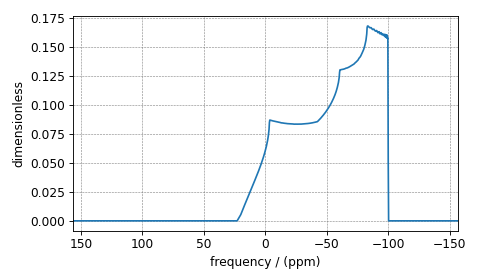
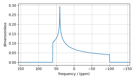
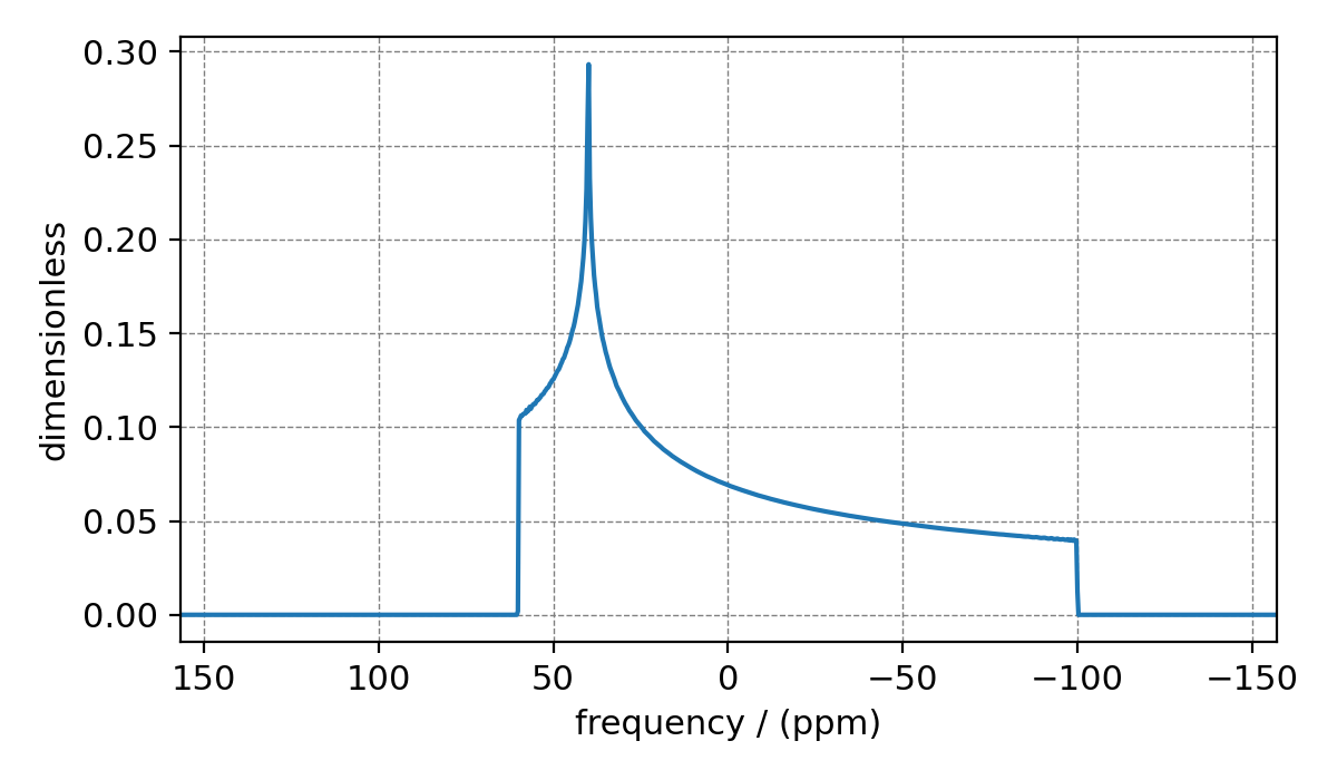
Figure 13 An example of an incomplete spectral averaging, where the simulation comprises of frequency contributions evaluated over the positive octant.
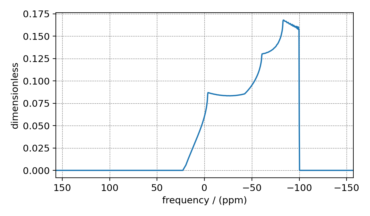
The spectrum in Figure 13 is incorrect. To fix this, set the integration volume to hemisphere and re-simulate. Figure 14 depicts the accurate simulation of the CSA tensor.
>>> # set integration volume to `hemisphere`.
>>> sim.config.integration_volume = 'hemisphere'
...
>>> # simulate and plot
>>> sim.run()
>>> plot(sim.methods[0].simulation)

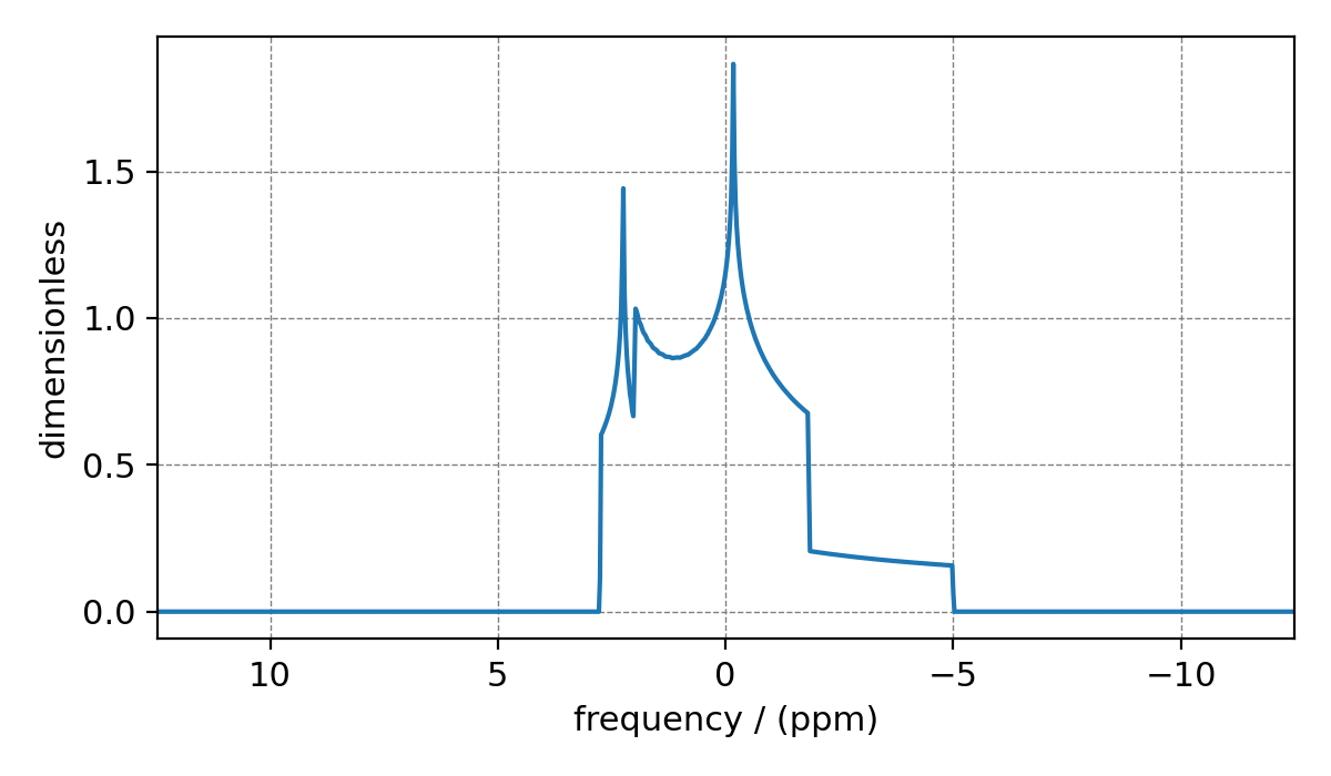
Figure 14 The spectrum resulting from the frequency contributions evaluated over the top hemisphere.
Integration density
Integration density controls the number of orientational points sampled over the given volume. The resulting spectrum is an integration of the NMR resonance frequency evaluated at these orientations. The total number of orientations, \(\Theta_\text{count}\), is given as
where \(M\) is the number of octants and \(n\) is value of this attribute. The number of octants is deciphered form the value of the integration_volume attribute. The default value of this attribute, 70, produces 2556 orientations at which the NMR frequency contribution is evaluated. The user may increase or decrease the value of this attribute as required by the problem.
Consider the following example.
>>> sim = Simulator()
>>> sim.config.integration_density
70
>>> sim.config.get_orientations_count() # 1 * 71 * 72 / 2
2556
>>> sim.config.integration_density = 100
>>> sim.config.get_orientations_count() # 1 * 101 * 102 / 2
5151
Decompose spectrum
The attribute decompose_spectrum is an enumeration with two literals, none,
and spin_system. The value of this attribute lets us know
how the user intends the simulation to be stored.
none
If the value is none (default), the result of the simulation is a single spectrum
where the frequency contributions from all the spin systems are co-added. Consider the
following example.
>>> # Create two sites
>>> site_A = Site(isotope='1H', shielding_symmetric={'zeta': 5, 'eta': 0.1})
>>> site_B = Site(isotope='1H', shielding_symmetric={'zeta': -2, 'eta': 0.83})
...
>>> # Create two spin systems, each with single site.
>>> system_A = SpinSystem(sites=[site_A], name='System-A')
>>> system_B = SpinSystem(sites=[site_B], name='System-B')
...
>>> # Create a method object.
>>> method = BlochDecaySpectrum(
...     channels=['1H'],
...     spectral_dimensions=[dict(count=1024, spectral_width=10000)]
... )
...
>>> # Create simulator object.
>>> sim = Simulator()
>>> sim.spin_systems += [system_A,  system_B] # add the spin systems
>>> sim.methods += [method] # add the method
...
>>> # simulate and plot.
>>> sim.run()
>>> plot(sim.methods[0].simulation)
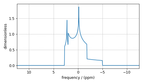
Figure 15 The spectrum is an integration of the spectra from individual spin systems when the
value of decompose_spectrum is none.
Figure 15 depicts the simulation of the spectrum from two spin systems where the contributions from individual spin systems are co-added.
spin_system
When the value of this attribute is spin_system, the resulting simulation is a
series of spectra, each arising from a spin system. In this case, the number of
spectra is the same as the number of spin system objects.
Try setting the value of the decompose_spectrum attribute to spin_system and observe
the simulation.
>>> # set decompose_spectrum to true.
>>> sim.config.decompose_spectrum = "spin_system"
...
>>> # simulate.
>>> sim.run()
...
>>> # plot of the two spectrum
>>> plot(sim.methods[0].simulation)
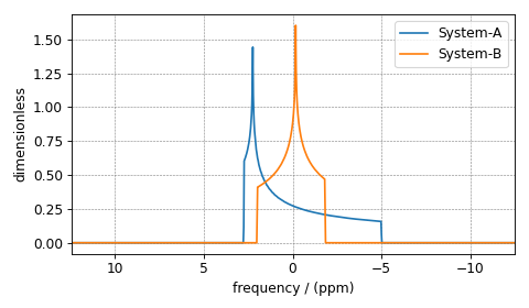
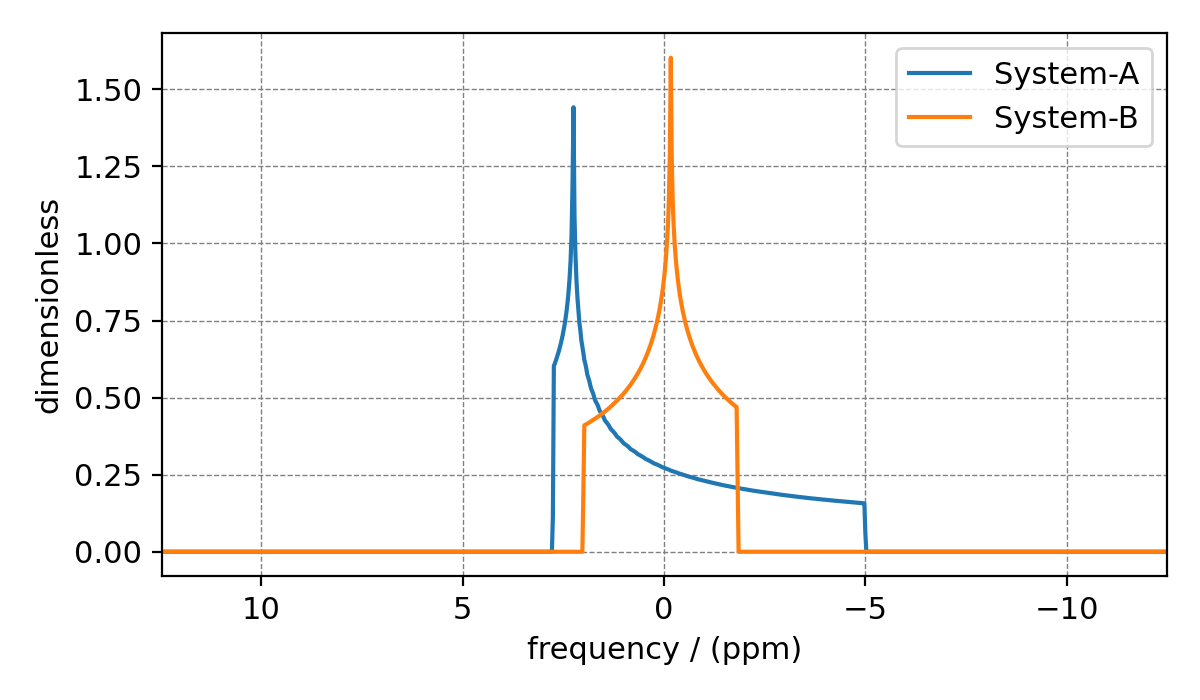
Figure 16 Spectrum from individual spin systems when the value of the decompose_spectrum
config is spin_system.
- 1
Edén, M. and Levitt, M. H. Computation of orientational averages in solid-state nmr by gaussian spherical quadrature. J. Mag. Res., 132, 2, 220–239, 1998. doi:10.1006/jmre.1998.1427.