
Signal Processing
Introduction
After running a simulation, you may need to apply some post-simulation signal processing.
For example, you may want to scale the intensities to match the experiment or convolve the
spectrum with a Lorentzian, Gaussian, or sinc line-broadening functions. There are many
signal-processing libraries, such as Numpy and Scipy, that you may use to accomplish this.
Although, in NMR, certain operations like convolutions, Fourier transform, and apodizations
are so regularly used that it soon becomes inconvenient to have to write your own set of
code. For this reason, the mrsimulator package offers some frequently used NMR signal
processing tools.
Note
The simulation object in mrsimulator is a CSDM object. A CSDM object is the python support for the core scientific dataset model (CSDM) 1, which is a new open-source universal file format for multi-dimensional datasets. Since CSDM objects hold a generic multi-dimensional scientific dataset, the following signal processing operation can be applied to any CSDM dataset, i.e., NMR, EPR, FTIR, GC, etc.
In the following section, we demonstrate the use of the
SignalProcessor class in applying various operations
to a generic CSDM object. But before we start explaining signal processing with CSDM
objects, it seems necessary to first describe the construct of CSDM objects. Each CSDM object
has two main attributes, dimensions and dependent_variables. The dimensions attribute
holds a list of Dimension objects, which collectively form a multi-dimensional Cartesian
coordinates grid system. A Dimension object can represent both physical and non-physical
dimensions. The dependent_variables attribute holds the responses of the multi-dimensional
grid points. You may have as many dependent variables as you like, as long as all dependent
variables share the same coordinates grid, i.e., dimensions.
SignalProcessor class
Signal processing is a series of operations that are applied to the dataset. In this workflow, the result from the previous operation becomes the input for the next operation.
In the mrsimulator library, all signal processing operations are accessed through the
signal_processing module. Within the module is the apodization sub-module. An
apodization is a point-wise multiplication operation of the input signal with the
apodizing vector. See Operations documentation for a complete list of
operations.
Import the module and sub-module as
>>> import mrsimulator.signal_processing as sp
>>> import mrsimulator.signal_processing.apodization as apo
Convolution
The convolution theorem states that under suitable conditions, the Fourier transform of a convolution of two signals is the pointwise product (apodization) of their Fourier transforms. In the following example, we employ this theorem to demonstrate how to apply a Gaussian convoluting to a dataset.
>>> processor = sp.SignalProcessor(
...     operations=[
...         sp.IFFT(), apo.Gaussian(FWHM='0.1 km'), sp.FFT()
...     ]
... )
Here, the processor is an instance of the SignalProcessor
class. The required attribute of this class, operations, is a list of operations. In the
above example, we employ the convolution theorem by sandwiching the Gaussian apodization
function between two Fourier transformations.
In this scheme, first, an inverse Fourier transform is applied to the datasets. On the resulting dataset, a Gaussian apodization, equivalent to a full width at half maximum of 0.1 km in the reciprocal dimension, is applied. The unit that you use for the FWHM attribute depends on the dimensionality of the dataset dimension. By choosing the unit as km, we imply that the corresponding dimension of the CSDM object undergoing the above series of operations has a dimensionality of length. Finally, a forward Fourier transform is applied to the apodized dataset.
Let’s create a CSDM object and then apply the above signal processing operations.
>>> import csdmpy as cp
>>> import numpy as np
...
>>> # Creating a test CSDM object.
>>> test_data = np.zeros(500)
>>> test_data[250] = 1
>>> csdm_object = cp.CSDM(
...     dependent_variables=[cp.as_dependent_variable(test_data)],
...     dimensions=[cp.LinearDimension(count=500, increment='1 m')]
... )
Note
See csdmpy for a detailed description of
generating CSDM objects. In mrsimulator, the simulation data is already stored as a
CSDM object.
To apply the previously defined signal processing operations to the above CSDM object, use
the apply_operations() method of the
SignalProcessor instance as follows,
>>> processed_data = processor.apply_operations(data=csdm_object)
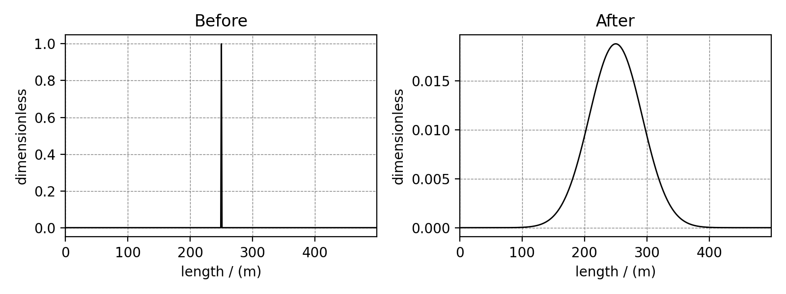
The data is the required argument of the apply_operations method, whose value is a CSDM object holding the dataset. The variable processed_data holds the output, that is, the processed data as a CSDM object. The plot of the original and the processed data is shown below.
>>> import matplotlib.pyplot as plt
>>> _, ax = plt.subplots(1, 2, figsize=(8, 3), subplot_kw={"projection":"csdm"})
>>> ax[0].plot(csdm_object, color="black", linewidth=1)
>>> ax[0].set_title('Before')
>>> ax[1].plot(processed_data.real, color="black", linewidth=1)
>>> ax[1].set_title('After')
>>> plt.tight_layout()
>>> plt.show()


Figure 17 The figure depicts an application of Gaussian convolution on a CSDM object.
Multiple convolutions
As mentioned before, a CSDM object may hold multiple dependent variables. When using the list of the operations, you may selectively apply a given operation to a specific dependent-variable by specifying the index of the corresponding dependent-variable as an argument to the operation class. Consider the following list of operations.
>>> processor = sp.SignalProcessor(
...     operations=[
...         sp.IFFT(),
...         apo.Gaussian(FWHM='0.1 km', dv_index=0),
...         apo.Exponential(FWHM='50 m', dv_index=1),
...         sp.FFT(),
...     ]
... )
The above signal processing operations first applies an inverse Fourier transform, followed by a Gaussian apodization on the dependent variable at index 0, followed by an Exponential apodization on the dependent variable at index 1, and finally a forward Fourier transform. Note, the FFT and IFFT operations apply on all dependent-variables.
Let’s add another dependent variable to the previously created CSDM object.
>>> # Add a dependent variable to the test CSDM object.
>>> test_data = np.zeros(500)
>>> test_data[150] = 1
>>> csdm_object.add_dependent_variable(cp.as_dependent_variable(test_data))
As before, apply the operations with the
apply_operations() method.
>>> processed_data = processor.apply_operations(data=csdm_object)
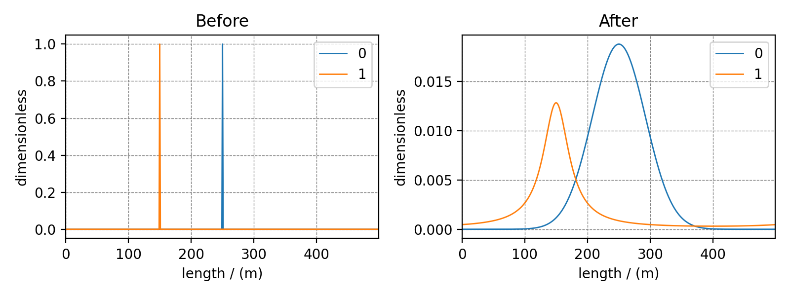
The plot of the dataset before and after signal processing is shown below.
>>> _, ax = plt.subplots(1, 2, figsize=(8, 3), subplot_kw={"projection":"csdm"})
>>> ax[0].plot(csdm_object, linewidth=1)
>>> ax[0].set_title('Before')
>>> ax[1].plot(processed_data.real, linewidth=1)
>>> ax[1].set_title('After')
>>> plt.tight_layout()
>>> plt.show()
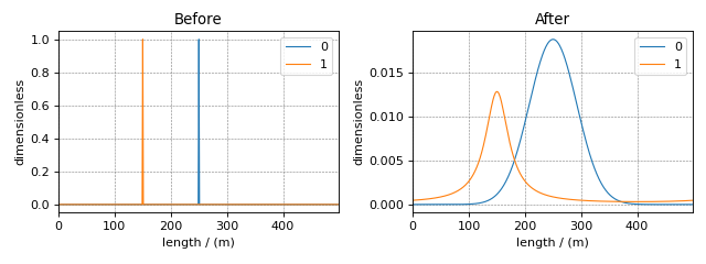
Figure 18 Gaussian and Lorentzian convolution applied to two different dependent variables of the CSDM object.
Convolution along multiple dimensions
In the case of multi-dimensional datasets, besides the dependent-variable index, you may also specify a dimension index along which a particular operation will apply. For example, consider the following 2D datasets as a CSDM object,
>>> # Create a two-dimensional CSDM object.
>>> test_data = np.zeros(600).reshape(30, 20)
>>> test_data[15, 10] = 1
>>> dv = cp.as_dependent_variable(test_data)
>>> dim1 = cp.LinearDimension(count=20, increment='0.1 ms', coordinates_offset='-1 ms', label='t1')
>>> dim2 = cp.LinearDimension(count=30, increment='1 cm/s', label='s1')
>>> csdm_data = cp.CSDM(dependent_variables=[dv], dimensions=[dim1, dim2])
where csdm_data is a two-dimensional dataset. Now consider the following signal processing
operations
>>> processor = sp.SignalProcessor(
...     operations=[
...         sp.IFFT(dim_index=(0, 1)),
...         apo.Gaussian(FWHM='0.5 ms', dim_index=0),
...         apo.Exponential(FWHM='10 cm/s', dim_index=1),
...         sp.FFT(dim_index=(0, 1)),
...     ]
... )
>>> processed_data = processor.apply_operations(data=csdm_data)
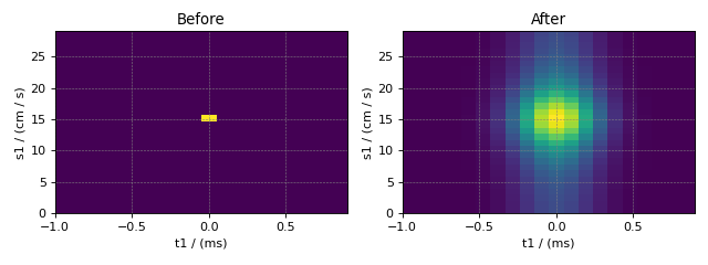
The above set of operations first performs an inverse FFT on the dataset along the dimension index 0 and 1. The second and third operations apply a Gaussian and Lorentzian apodization along dimensions 0 and 1, respectively. The last operation is a forward Fourier transform. The before and after plots of the datasets are shown below.
>>> _, ax = plt.subplots(1, 2, figsize=(8, 3), subplot_kw={"projection":"csdm"})
>>> ax[0].imshow(csdm_data, aspect='auto')
>>> ax[0].set_title('Before')
>>> ax[1].imshow(processed_data.real, aspect='auto')
>>> ax[1].set_title('After')
>>> plt.tight_layout()
>>> plt.show()

Serializing the operations list
You may also serialize the operations list using the
json()
method, as follows
>>> from pprint import pprint
>>> pprint(processor.json())
{'operations': [{'dim_index': [0, 1], 'function': 'IFFT'},
                {'FWHM': '0.5 ms',
                 'dim_index': 0,
                 'function': 'apodization',
                 'type': 'Gaussian'},
                {'FWHM': '10.0 cm / s',
                 'dim_index': 1,
                 'function': 'apodization',
                 'type': 'Exponential'},
                {'dim_index': [0, 1], 'function': 'FFT'}]}
- 1
Srivastava, D. J., Vosegaard, T., Massiot, D., Grandinetti, P. J., Core Scientific Dataset Model: A lightweight and portable model and file format for multi-dimensional scientific data, PLOS ONE, 15, 1-38, (2020). DOI:10.1371/journal.pone.0225953
See also
Simulation Examples for application of signal processing on NMR simulations.