
Czjzek distribution
A Czjzek distribution model is a random distribution of the second-rank traceless symmetric tensors about a zero tensor. See Czjzek distribution and references within for a brief description of the model.
Czjzek distribution of symmetric shielding tensors
To generate a Czjzek distribution, use the CzjzekDistribution
class as follows.
>>> from mrsimulator.models import CzjzekDistribution
>>> cz_model = CzjzekDistribution(sigma=0.8)
The CzjzekDistribution class accepts a single argument, sigma, which is the standard
deviation of the second-rank traceless symmetric tensor parameters. In the above example,
we create cz_model as an instance of the CzjzekDistribution class with
\(\sigma=0.8\).
Note, cz_model is only a class instance of the Czjzek distribution. You can either
draw random points from this distribution or generate a probability distribution
function. Let’s first draw points from this distribution, using the
rvs() method of the instance.
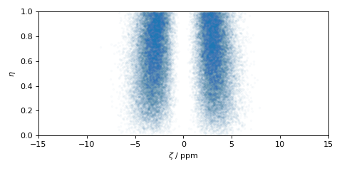
>>> zeta_dist, eta_dist = cz_model.rvs(size=50000)
In the above example, we draw size=50000 random points of the distribution. The output
zeta_dist and eta_dist hold the tensor parameter coordinates of the points, defined
in the Haeberlen convention.
The scatter plot of these coordinates is shown below.
>>> import matplotlib.pyplot as plt
>>> plt.scatter(zeta_dist, eta_dist, s=4, alpha=0.02)
>>> plt.xlabel('$\zeta$ / ppm')
>>> plt.ylabel('$\eta$')
>>> plt.xlim(-15, 15)
>>> plt.ylim(0, 1)
>>> plt.tight_layout()
>>> plt.show()

Czjzek distribution of symmetric quadrupolar tensors
The Czjzek distribution of symmetric quadrupolar tensors follows a similar setup as the
Czjzek distribution of symmetric shielding tensors, except we assign the outputs to Cq
and \(\eta_q\). In the following example, we generate the probability distribution
function using the pdf() method.
>>> import numpy as np
>>> Cq_range = np.arange(100)*0.3 - 15 # pre-defined Cq range in MHz.
>>> eta_range = np.arange(21)/20  # pre-defined eta range.
>>> Cq, eta, amp = cz_model.pdf(pos=[Cq_range, eta_range])
To generate a probability distribution, we need to define a grid system over which the
distribution probabilities will be evaluated. We do so by defining the range of coordinates
along the two dimensions. In the above example, Cq_range and eta_range are the
range of \(\text{Cq}\) and \(\eta_q\) coordinates, which is then given as the
argument to the pdf() method. The output
Cq, eta, and amp hold the two coordinates and amplitude, respectively.
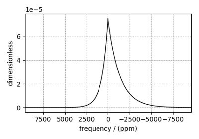
The plot of the Czjzek probability distribution is shown below.
>>> import matplotlib.pyplot as plt
>>> plt.contourf(Cq, eta, amp, levels=10)
>>> plt.xlabel('$C_q$ / MHz')
>>> plt.ylabel('$\eta$')
>>> plt.tight_layout()
>>> plt.show()

Note
The pdf method of the instance generates the probability distribution function
by first drawing random points from the distribution and then binning it
onto a pre-defined grid.
Mini-gallery using the Czjzek distributions

Figure 20 Czjzek distribution, 27Al (I=5/2) 3QMAS