Getting started with mrsimulator: Using objects

In the previous section on getting started, we show an example where we parse the python dictionaries to create instances of the SpinSystem and Method objects. In this section, we’ll illustrate how we can achieve the same result using the core mrsimulator objects.

Note

Unlike python dictionary objects from our last example, when using mrsimulator objects, the attribute value is given as a number rather than a string with a number and a unit. We assume default units for the class attributes. To learn more about the default units, please refer to the documentation of the respective class. For the convenience of our users, we have added an attribute, property_units, to every class that holds the default unit of the respective class attributes.

Let’s start by importing the classes.

>>> from mrsimulator import Simulator, SpinSystem, Site
>>> from mrsimulator.methods import BlochDecaySpectrum

---

The following code is used to produce the figures in this section.

>>> import matplotlib.pyplot as plt
>>> import matplotlib as mpl
>>> mpl.rcParams["figure.figsize"] = (6, 3.5)
>>> mpl.rcParams["font.size"] = 11
...
>>> # function to render figures.
>>> def plot(csdm_object):
...     # set matplotlib axes projection='csdm' to directly plot CSDM objects.
...     ax = plt.subplot(projection='csdm')
...     ax.plot(csdm_object, linewidth=1.5)
...     ax.invert_xaxis()
...     plt.tight_layout()
...     plt.show()

---

Site object

As the name suggests, a Site object is used in creating sites. For example,

>>> C13A = Site(isotope='13C')

The above code creates a site with a \(^{13}\text{C}\) isotope. Because, no further information is delivered to the site object, other attributes such as the isotropic chemical shift assume their default value.

>>> C13A.isotropic_chemical_shift # value is given in ppm
0

Here, the isotropic chemical shift is given in ppm. This information is also present in the property_units attribute of the instance. For example,

>>> C13A.property_units
{'isotropic_chemical_shift': 'ppm'}

Let’s create a few more sites.

>>> C13B = Site(isotope='13C', isotropic_chemical_shift=-10)
>>> H1 = Site(isotope='1H', shielding_symmetric=dict(zeta=5.1, eta=0.1))
>>> O17 = Site(isotope='17O', isotropic_chemical_shift=41.7, quadrupolar=dict(Cq=5.15e6, eta=0.21))

The site, C13B, is the second \(^{13}\text{C}\) site with an isotropic chemical shift of -10 ppm.

In creating the site, H1, we use the dictionary object to describe a traceless symmetric second-rank irreducible nuclear shielding tensor, using the attributes zeta and eta, respectively. The parameter zeta and eta are defined as per the Haeberlen convention and describes the anisotropy and asymmetry parameter of the tensor, respectively. The default unit of the attributes from the shielding_symmetric is found with the property_units attribute, such as

>>> H1.shielding_symmetric.property_units
{'zeta': 'ppm', 'alpha': 'rad', 'beta': 'rad', 'gamma': 'rad'}

For site, O17, we once again make use of the dictionary object, only this time to describe a traceless symmetric second-rank irreducible electric quadrupole tensor, using the attributes Cq and eta, respectively. The parameter Cq is the quadrupole coupling constant, and eta is the asymmetry parameters of the quadrupole tensor, respectively. The default unit of these attributes is once again found with the property_units attribute,

>>> O17.quadrupolar.property_units
{'Cq': 'Hz', 'alpha': 'rad', 'beta': 'rad', 'gamma': 'rad'}

SpinSystem object

A SpinSystem object contains sites and couplings along with the abundance of the respective spin system. In this version, we focus on the spin systems with a single site, and therefore the couplings are irrelevant.

Let’s use the sites we have already created to set up four spin systems.

>>> system_1 = SpinSystem(name='C13A', sites=[C13A], abundance=20)
>>> system_2 = SpinSystem(name='C13B', sites=[C13B], abundance=56)
>>> system_3 = SpinSystem(name='H1', sites=[H1], abundance=100)
>>> system_4 = SpinSystem(name='O17', sites=[O17], abundance=1)

Method object

Likewise, we can create a BlochDecaySpectrum object following,

>>> from mrsimulator.methods import BlochDecaySpectrum
>>> method_1 = BlochDecaySpectrum(
...     channels=["13C"],
...     spectral_dimensions = [dict(
...         count=2048,
...         spectral_width=25000, # in Hz.
...         label=r"$^{13}$C resonances",
...     )]
... )

The above method, method_1, is defined to record \(^{13}\text{C}\) resonances over 25 kHz spectral width using 2048 points. The unspecified attributes, such as rotor_frequency, rotor_angle, magnetic_flux_density, assume their default value. The default units of these attributes is once again found with the property_units attribute,

>>> method_1.property_units
{'magnetic_flux_density': 'T', 'rotor_angle': 'rad', 'rotor_frequency': 'Hz'}

Simulator object

The use of the simulator object is the same as described in the previous section.

>>> sim = Simulator()
>>> sim.spin_systems += [system_1, system_2, system_3, system_4] # add the spin systems
>>> sim.methods += [method_1] # add the method

Running simulation

Let’s run the simulator and observe the spectrum.

>>> sim.run()
>>> plot(sim.methods[0].simulation) 

(png, hires.png, pdf)

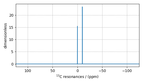
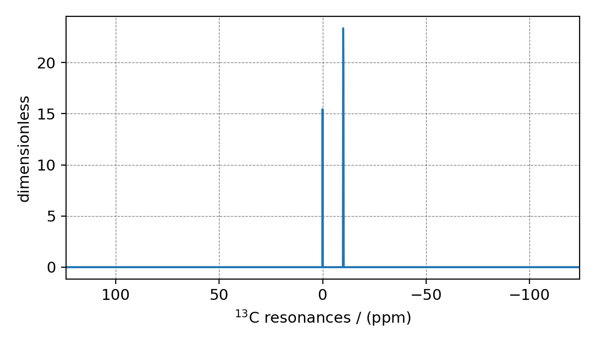
Figure 3 An example solid-state NMR simulation of \(^{13}\text{C}\) isotropic spectrum.

Notice, we have four single-site spin systems within the sim object, two with \(^{13}\text{C}\) sites, one with \(^1\text{H}\) site, and one with an \(^{17}\text{O}\) site, along with a BlochDecaySpectrum method which is tuned to record the resonances from the \(^{13}\text{C}\) channel. When you run this simulation, only \(^{13}\text{C}\) resonances are recorded, as seen from Figure 3, where just the two \(^{13}\text{C}\) isotropic chemical shifts resonances are observed.

Modifying the site attributes

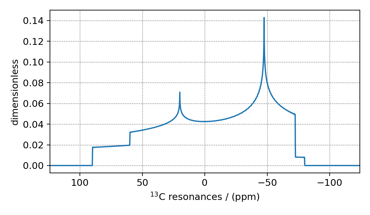
Let’s modify the C13A and C13B sites by adding the shielding tensors information.

>>> sim.spin_systems[0].sites[0].shielding_symmetric = dict(zeta=80, eta=0.5) # site C13A
>>> sim.spin_systems[1].sites[0].shielding_symmetric = dict(zeta=-100, eta=0.25) # site C13B

Running the simulation with the previously defined method will produce two overlapping CSA patterns, see Figure 4.

>>> sim.run()
>>> plot(sim.methods[0].simulation) 

(png, hires.png, pdf)

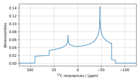
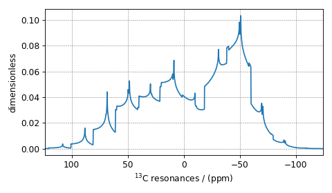
Figure 4 An example state-solid NMR simulation of static \(^{13}\text{C}\) CSA spectrum.

Modifying the rotor frequency of the method

Let’s turn up the rotor frequency from 0 Hz (default) to 1 kHz. Note, that we do not add another method to the sim object, but update the existing method at index 0 with a new method. Figure 5 depicts the simulation from this method.

>>> # Update the method object at index 0.
>>> sim.methods[0] = BlochDecaySpectrum(
...     channels=["13C"],
...     rotor_frequency=1000, # in Hz.  <------------ updated entry
...     spectral_dimensions=[dict(
...         count=2048,
...         spectral_width=25000, # in Hz.
...         label=r"$^{13}$C resonances",
...     )]
... )

>>> sim.run()
>>> plot(sim.methods[0].simulation) 

(png, hires.png, pdf)

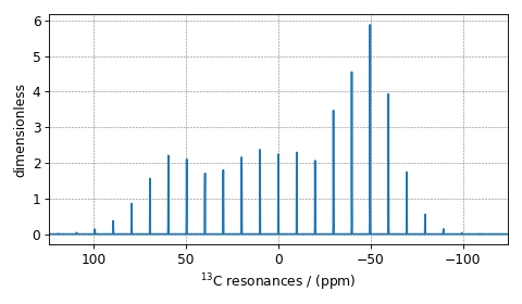
Figure 5 An example of the solid-state \(^{13}\text{C}\) MAS sideband simulation.

Modifying the rotor angle of the method

Let’s also set the rotor angle from magic angle (default) to 90 degrees. Again, we update the method at index 0. Figure 6 depicts the simulation from this method.

>>> # Update the method object at index 0.
>>> sim.methods[0] = BlochDecaySpectrum(
...     channels=["13C"],
...     rotor_frequency=1000, # in Hz.
...     rotor_angle=90*3.1415926/180, # 90 degree in radians.  <------------ updated entry
...     spectral_dimensions=[dict(
...         count=2048,
...         spectral_width=25000, # in Hz.
...         label=r"$^{13}$C resonances",
...     )]
... )

>>> sim.run()
>>> plot(sim.methods[0].simulation) 

(png, hires.png, pdf)

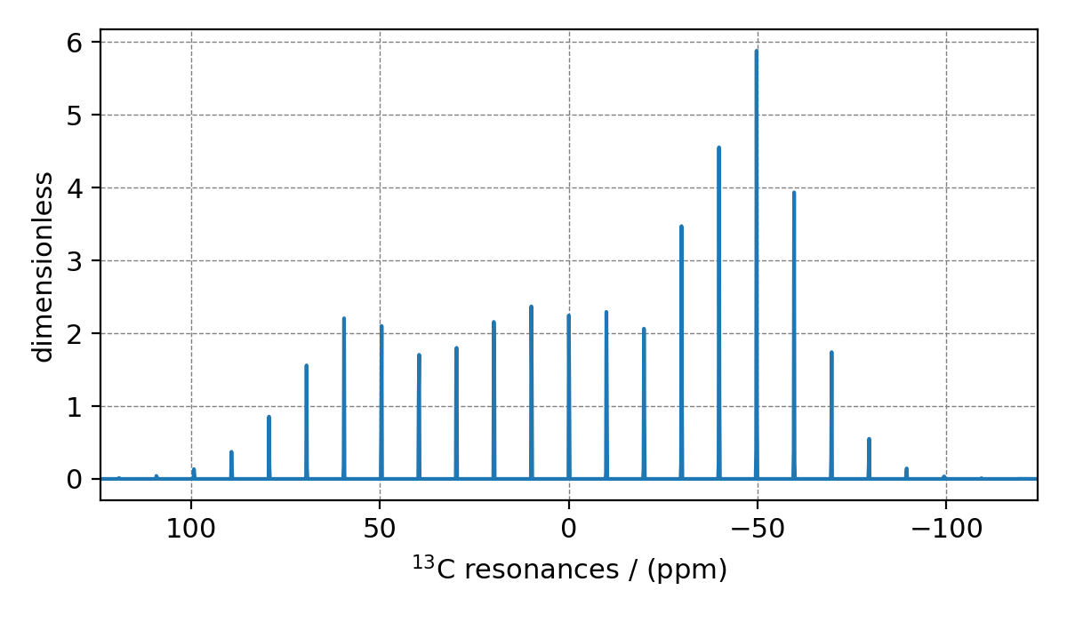
Figure 6 An example of the solid-state \(^{13}\text{C}\) VAS sideband simulation.

Switching the detection channels of the method

To switch to another channels, update the value of the channels attribute of the method. Here, we update the method to 1H channel.

>>> # Update the method object at index 0.
>>> sim.methods[0] = BlochDecaySpectrum(
...     channels=["1H"], # <------------ updated entry
...     rotor_frequency=1000, # in Hz.
...     rotor_angle=90*3.1415926/180, # 90 degree in radians.
...     spectral_dimensions=[dict(
...         count=2048,
...         spectral_width=25000, # in Hz.
...         label=r"$^1$H resonances",
...     )]
... )

>>> sim.run()
>>> plot(sim.methods[0].simulation) 

(png, hires.png, pdf)

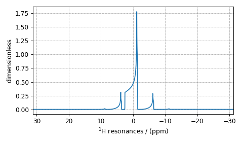
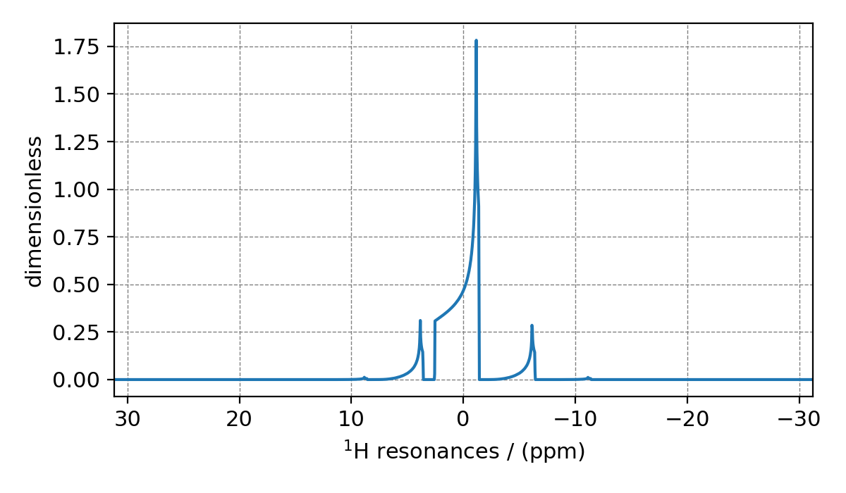
Figure 7 An example of solid-state \(^{1}\text{H}\) VAS sideband simulation.

In Figure 7, we see a \(90^\circ\) spinning sideband \(^1\text{H}\)-spectrum, whose frequency contributions arise from system_3 because system_3 is the only spin system with \(^1\text{H}\) site.

Note, although you are free to assign any channel to the channels attribute of the BlochDecaySpectrum method, only channels whose isotopes are also a member of the spin systems will produce a spectrum. For example, the following method

>>> # Update the method object at index 0.
>>> sim.methods[0] = BlochDecaySpectrum(
...     channels=["23Na"], # <------------ updated entry
...     rotor_frequency=1000, # in Hz.
...     rotor_angle=90*3.1415926/180, # 90 degree in radians.
...     spectral_dimensions=[dict(
...         count=2048,
...         spectral_width=25000, # in Hz.
...         label=r"$^{23}$Na resonances",
...     )]
... )

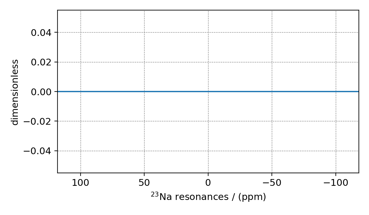
is defined to collect the resonances from \(^{23}\text{Na}\) isotope. As you may have noticed, we do not have any \(^{23}\text{Na}\) site in the spin systems. Simulating the spectrum from this method will result in a zero amplitude spectrum, see Figure 8.

>>> sim.run()
>>> plot(sim.methods[0].simulation) 

(png, hires.png, pdf)

Figure 8 An example of a simulation where the isotope from the method’s channel attribute does not exist within the spin systems.

Switching the channel to 17O

Likewise, update the value of the channels attribute to 17O.

>>> sim.methods[0] = BlochDecaySpectrum(
...     channels=["17O"],
...     rotor_frequency= 15000, # in Hz.
...     rotor_angle = 0.9553166, # magic angle is rad.
...     spectral_dimensions=[dict(
...         count=2048,
...         spectral_width=25000, # in Hz.
...         label=r"$^{17}$O resonances",
...     )]
... )
>>> sim.run()
>>> plot(sim.methods[0].simulation) 

(png, hires.png, pdf)

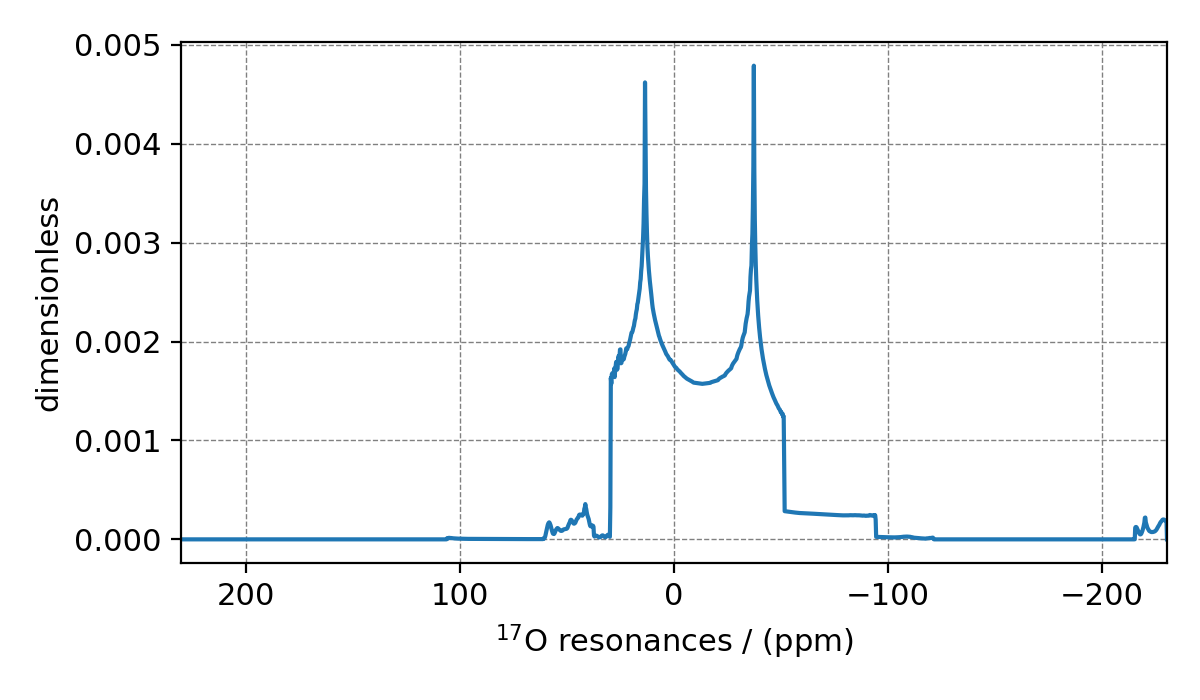
Figure 9 An example of the solid-state \(^{17}\text{O}\) BlochDecaySpectrum simulation.

If you are familiar with the quadrupolar line-shapes, you may immediately associate the spectrum in Figure 9 to a second-order quadrupolar line-shape of the central transition. You may also notice some unexpected resonances around 50 ppm and -220 ppm. These unexpected resonances are the spinning sidebands of the satellite transitions. Note, the BlochDecaySpectrum method computes resonances from all transitions with \(p = \Delta m = -1\).

Let’s see what transition pathways are used in our simulation. Use the get_transition_pathways() function of the Method instance to see the list of transition pathways, for example,

>>> from pprint import pprint
>>> pprint(sim.methods[0].get_transition_pathways(system_4)) # 17O
[TransitionPathway(|-2.5⟩⟨-1.5|),
 TransitionPathway(|-1.5⟩⟨-0.5|),
 TransitionPathway(|-0.5⟩⟨0.5|),
 TransitionPathway(|0.5⟩⟨1.5|),
 TransitionPathway(|1.5⟩⟨2.5|)]

Notice, there are five transition pathways for the \(^{17}\text{O}\) site, one associated with the central-transition, two with the inner-satellites, and two with the outer-satellites. For central transition selective simulation, use the BlochDecayCentralTransitionSpectrum method.

>>> from mrsimulator.methods import BlochDecayCentralTransitionSpectrum
>>> sim.methods[0] = BlochDecayCentralTransitionSpectrum(
...     channels=["17O"],
...     rotor_frequency= 15000, # in Hz.
...     rotor_angle = 0.9553166, # magic angle is rad.
...     spectral_dimensions=[dict(
...         count=2048,
...         spectral_width=25000, # in Hz.
...         label=r"$^{17}$O resonances",
...     )]
... )
>>> # the transition pathways
>>> print(sim.methods[0].get_transition_pathways(system_4)) # 17O
[TransitionPathway(|-0.5⟩⟨0.5|)]

Now, you may simulate the central transition selective spectrum. Figure 10 depicts a central transition selective spectrum.

>>> sim.run()
>>> plot(sim.methods[0].simulation) 

(png, hires.png, pdf)

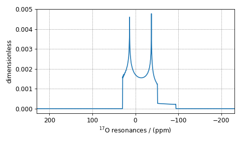
Figure 10 An example of the solid-state \(^{17}\text{O}\) BlochDecayCentralTransitionSpectrum simulation.