Getting started with mrsimulator: The basics

We have put together a set of guidelines for using the mrsimulator package. We encourage our users to follow these guidelines for consistency. In mrsimulator, the solid-state nuclear magnetic resonance (ssNMR) spectrum is calculated through an instance of the Simulator class.

Import the Simulator class using

>>> from mrsimulator import Simulator

and create an instance as follows,

>>> sim = Simulator()

Here, the variable sim is an instance of the Simulator class. The two attributes of this class that you will frequently use are the spin_systems and methods, whose values are a list of SpinSystem and Method objects, respectively. The default value of these attributes is an empty list.

>>> sim.spin_systems
[]
>>> sim.methods
[]

Before you can start simulating the NMR spectrum, you need to understand the role of the SpinSystem and Method objects. The following provides a brief description of the respective objects.

Setting up the SpinSystem objects

An NMR spin system is an isolated system of sites (spins) and couplings. You may construct a spin system with as many sites and couplings, as necessary, for this example, we stick to a single-site spin system. Let’s start by first building a site.

A site object is a collection of attributes that describe site-specific interactions. In NMR, these spin interactions are described by a second-rank tensor. Site-specific interactions include the interaction between the magnetic dipole moment of the nucleus and the surrounding magnetic field and the interaction between the electric quadrupole moment of the nucleus with the surrounding electric field gradient. The latter is zero for sites with the spin quantum number, \(I=1/2\).

Let’s start with a spin-1/2 isotope, \(^{29}\text{Si}\), and create a site.

>>> the_site = {
...     "isotope": "29Si",
...     "isotropic_chemical_shift": "-101.1 ppm",
...     "shielding_symmetric": {"zeta": "70.5 ppm", "eta": 0.5},
... }

In the above code, the_site is a simplified python dictionary representation of a Site object. This site describes a \(^{29}\text{Si}\) isotope with a -101.1 ppm isotropic chemical shift along with the symmetric part of the nuclear shielding anisotropy tensor, described here with the parameters zeta and eta using the Haeberlen convention.

That’s it! Now that we have a site, we can create a single-site spin system following,

>>> the_spin_system = {
...     "name": "site A",
...     "description": "A test 29Si site",
...     "sites": [the_site],  # from the above code
...     "abundance": "80%",
... }

As mentioned before, a spin system is a collection of sites and couplings. In the above example, we have created a spin system with a single site and no couplings. Here, the attribute sites hold a list of sites. The attributes name, description, and abundance are optional.

Until now, we have only created a python dictionary representation of a spin system. To run the simulation, you need to create an instance of the SpinSystem class. Import the SpinSystem class and use it’s parse_dict_with_units() method to parse the python dictionary and create an instance of the spin system class, as follows,

>>> from mrsimulator import SpinSystem
>>> system_object_1 = SpinSystem.parse_dict_with_units(the_spin_system)

Note

We provide the parse_dict_with_units() method because it allows the user to create spin systems, where the attribute value is a physical quantity, represented as a string with a value and a unit. Physical quantities remove the ambiguity in the units, which is otherwise a source of general confusion within many scientific applications. With this said, parsing physical quantities can add significant overhead when used in an iterative algorithm, such as the least-squares minimization. In such cases, we recommend defining objects directly. See the Getting started with mrsimulator: Using objects for details.

We have successfully created a spin system object. To create more spin system objects, repeat the above set of instructions. In this example, we stick with a single spin system object. Once all spin system objects are ready, add these objects to the instance of the Simulator class, as follows

>>> sim.spin_systems += [system_object_1] # add all spin system objects.

Setting up the Method objects

A Method object is a collection of attributes that describe an NMR method. In mrsimulator, all methods are described through five keywords -

Keywords	Description
channels	A list of isotope symbols over which the given method applies.
magnetic_flux_density	The macroscopic magnetic flux density of the applied external magnetic field.
rotor_angle	The angle between the sample rotation axis and the applied external magnetic field.
rotor_frequency	The sample rotation frequency.
spectral_dimensions	A list of spectral dimensions. The coordinates along each spectral dimension is described with the keywords, count (\(N\)), spectral_width (\(\nu_\text{sw}\)), and reference_offset (\(\nu_0\)). The coordinates are given as, (1)\[\left([0, 1, 2, ... N-1] - \frac{T}{2}\right) \frac{\nu_\text{sw}}{N} + \nu_0\] where \(T=N\) when \(N\) is even else \(T=N-1\).

Let’s start with the simplest method, the BlochDecaySpectrum(). The following is a python dictionary representation of the BlochDecaySpectrum method.

>>> method_dict = {
...     "channels": ["29Si"],
...     "magnetic_flux_density": "9.4 T",
...     "rotor_angle": "54.735 deg",
...     "rotor_frequency": "0 Hz",
...     "spectral_dimensions": [{
...         "count": 2048,
...         "spectral_width": "25 kHz",
...         "reference_offset": "-8 kHz",
...         "label": r"$^{29}$Si resonances",
...     }]
... }

Here, the key channels is a list of isotope symbols over which the method is applied. A Bloch Decay method only has a single channel. In this example, it is given a value of 29Si, which implies that the simulated spectrum from this method will comprise frequency components arising from the \(^{29}\text{Si}\) resonances. The keys magnetic_flux_density, rotor_angle, and rotor_frequency collectively describe the spin environment under which the resonance frequency is evaluated. The key spectral_dimensions is a list of spectral dimensions. A Bloch Decay method only has one spectral dimension. In this example, the spectral dimension defines a frequency dimension with 2048 points, spanning for 25 kHz with a reference offset of -8 kHz.

Like before, you may parse the above method_dict using the parse_dict_with_units() function of the method. Import the BlochDecaySpectrum class and create an instance of the method, following,

>>> from mrsimulator.methods import BlochDecaySpectrum
>>> method_object = BlochDecaySpectrum.parse_dict_with_units(method_dict)

Here, method_object, is an instance of the Method class.

Likewise, you may create multiple method objects. In this example, we stick with a single method. Finally, add all the method objects, in this case, method_object, to the instance of the Simulator class, sim, as follows,

>>> sim.methods += [method_object] # add all methods.

Running simulation

To simulate the spectrum, run the simulator with the run() method, as follows,

>>> sim.run()

Note

In mrsimulator, all resonant frequencies are calculated assuming the weakly-coupled (Zeeman) basis for the spin system.

The simulator object, sim, will process every method over all the spin systems and store the result in the simulation attribute of the respective Method object. In this example, we have a single method. You may access the simulation data for this method as,

>>> data_0 = sim.methods[0].simulation
>>> # data_n = sim.method[n].simulation # when there are multiple methods.

Here, data_0 is a CSDM object holding the simulation data from the method at index 0 of the methods attribute from the sim object.

See also

The core scientific dataset model (CSDM) 1 is a lightweight and portable file format model for multi-dimensional scientific datasets and is supported by numerous NMR software—DMFIT, SIMPSON, jsNMR, and RMN. We also provide a python package csdmpy.

Visualizing the dataset

At this point, you may continue with additional post-simulation processing. We end this example with a plot of the data from the simulation. Figure 2 depicts the plot of the simulated spectrum.

For a quick plot of the csdm data, you may use the csdmpy library. The csdmpy package uses the matplotlib library to produce basic plots. You may optionally customize the plot using matplotlib methods.

>>> import matplotlib.pyplot as plt
>>> plt.figure(figsize=(6, 3.5)) # set the figure size 
>>> ax = plt.subplot(projection='csdm') 
>>> ax.plot(data_0) 
>>> ax.invert_xaxis() # reverse x-axis 
>>> plt.tight_layout(pad=0.1) 
>>> plt.show() 

(png, hires.png, pdf)

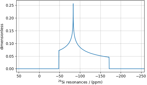
Figure 2 An example of solid-state static NMR spectrum simulation.

1

Srivastava, D. J., Vosegaard, T., Massiot, D., Grandinetti, P. J. Core Scientific Dataset Model: A lightweight and portable model and file format for multi-dimensional scientific data. PLOS ONE, 2020, 15, 1. DOI 10.1371/e0225953