Isotopomers Example

Here, you will work through an example that should be familiar to nearly all practitioners of NMR spectroscopy, i.e., the simulation of the \(^1\text {H}\) and \(^{13}\text{C}\) liquid-state NMR spectra of ethanol with its various isotopomers. The \(^1\text{H}\) spectrum will include the characteristic \(^{13}\text{C}\) satellite peaks which arise from couplings between \(^{1}\text{H}\) and \(^{13}\text{C}\) in low-abundance isotopomers.

Spin Systems

The molecules in a sample of ethanol, \(\text{CH$_3$CH$_2$OH}\), can be formed with any of the naturally abundant isotopes of hydrogen, carbon, and oxygen present. Of the most abundant isotopes, \(^1\text{H}\) (99.985%), \(^{12}\text{C}\) (98.93%), and \(^ {16}\text{O}\) (99.762%), only \(^1\text{H}\) is NMR active. The most abundant NMR active isotopes of carbon and oxygen are \(^{13}\text{C}\) (1.11%) and \(^{17}\text{O}\) (0.038%). Additionally, the \(^2\text{H}\) (0.015%) isotope will be present. For our purposes, we will ignore the effects of the lower abundant \(^{17}\text {O}\) and \(^2\text{H}\) isotopes, and focus solely on the spectra of the isotopomers formed from \(^1\text{H}\), \(^{12}\text {C}\) , and \(^{13}\text{C}\). This leaves us with the three most abundant isotopomers of ethanol shown below.

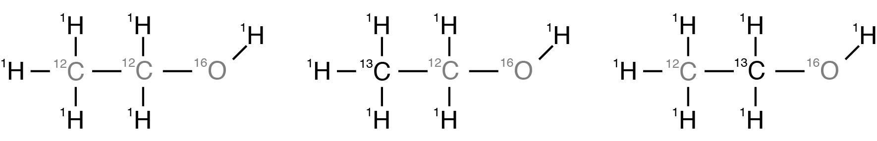
Figure 7 The three most abundant isotopomers of ethanol.

The most abundant isotopomer, on the left, has a probability of \((0.99985)^6 \times (0.9893)^2 \times (0.99762) =0.9625\), while the last two have identical probabilities of \((0.99985)^6 \times (0.0111) (0.9893) \times (0.99762) = 0.0108\)

Before you can construct spin systems for each of these isotopomers, you’ll need to create sites for each of the three magnetically inequivalent \(^1\text{H}\) and two magnetically inequivalent \(^{13}\text{C}\) sites, as shown in the code below.

from mrsimulator import Simulator, Site, SpinSystem, Coupling

# All shifts in ppm
# methyl proton site
H_CH3 = Site(isotope="1H", isotropic_chemical_shift=1.226)
# methylene proton site
H_CH2 = Site(isotope="1H", isotropic_chemical_shift=2.61)
# hydroxyl proton site
H_OH = Site(isotope="1H", isotropic_chemical_shift=3.687)

# methyl carbon site
C_CH3 = Site(isotope="13C", isotropic_chemical_shift=18)
# methylene carbon site
C_CH2 = Site(isotope="13C", isotropic_chemical_shift=58)

These sites will be used, along with Coupling instances described below, to create each of the isotopomers.

Isotopomer 1

To create the SpinSystem instance for the most abundant isotopomer, start by creating a list of sites present in this isotopomer.

# Put sites into list
iso1_sites = [H_CH3, H_CH3, H_CH3, H_CH2, H_CH2, H_OH]

Each site in the isotopomer is identified by its index in the iso1_sites ordered list, which are numbered from 0 to 5. Remember that the two Sites involved in a Coupling are identified by their indexes in this list.

Next, create the Coupling instances between the sites and place the Coupling instances in a list.

# All isotropic_j coupling in Hz
HH_coupling_1 = Coupling(site_index=[0, 3], isotropic_j=7)
HH_coupling_2 = Coupling(site_index=[0, 4], isotropic_j=7)
HH_coupling_3 = Coupling(site_index=[1, 3], isotropic_j=7)
HH_coupling_4 = Coupling(site_index=[1, 4], isotropic_j=7)
HH_coupling_5 = Coupling(site_index=[2, 3], isotropic_j=7)
HH_coupling_6 = Coupling(site_index=[2, 4], isotropic_j=7)

# Put couplings into list
iso1_couplings = [
    HH_coupling_1,
    HH_coupling_2,
    HH_coupling_3,
    HH_coupling_4,
    HH_coupling_5,
    HH_coupling_6,
]

Finally, create the SpinSystem instance for this isotopomer along with its abundance.

isotopomer1 = SpinSystem(sites=iso1_sites, couplings=iso1_couplings, abundance=96.25)

Isotopomer 2

Replacing the methyl carbon with a \(^{13}\text{C}\) isotope gives the second isotopomer. To create its SpinSystem instance, follow the code below, where (1) you create the list of sites to include the C_CH3 site, (2) you create three Coupling instances for its J coupling to the three attached protons, (3) you create the list of couplings, and, finally, (4) you create the SpinSystem instance for the isotopomer using the lists of sites and couplings along with the isotopomer’s abundance of 1.08%.

# Put sites into list
iso2_sites = [H_CH3, H_CH3, H_CH3, H_CH2, H_CH2, H_OH, C_CH3]

# Define methyl 13C - 1H couplings
CH3_coupling_1 = Coupling(site_index=[0, 6], isotropic_j=125)
CH3_coupling_2 = Coupling(site_index=[1, 6], isotropic_j=125)
CH3_coupling_3 = Coupling(site_index=[2, 6], isotropic_j=125)

# Add new couplings to existing 1H - 1H couplings
iso2_couplings = iso1_couplings + [CH3_coupling_1, CH3_coupling_2, CH3_coupling_3]

isotopomer2 = SpinSystem(sites=iso2_sites, couplings=iso2_couplings, abundance=1.08)

Isotopomer 3

Lastly, build the sites, couplings, and spin system for the isotopomer with the methylene carbon replaced with a \(^{13}\text{C}\) isotope.

# Put sites into list
iso3_sites = [H_CH3, H_CH3, H_CH3, H_CH2, H_CH2, H_OH, C_CH2]

# Define methylene 13C - 1H couplings
CH2_coupling_1 = Coupling(site_index=[3, 6], isotropic_j=141)
CH2_coupling_2 = Coupling(site_index=[4, 6], isotropic_j=141)

# Add new couplings to existing 1H - 1H couplings
iso3_couplings = iso1_couplings + [CH2_coupling_1, CH2_coupling_2]

isotopomer3 = SpinSystem(sites=iso3_sites, couplings=iso3_couplings, abundance=1.08)

Methods

For this example, create two BlochDecaySpectrum methods for \(^1\text {H}\) and \(^{13}\text{C}\). Recall that this method simulates the spectrum for the first isotope in the channels attribute list.

from mrsimulator.method.lib import BlochDecaySpectrum
from mrsimulator.method import SpectralDimension

method_H = BlochDecaySpectrum(
    channels=["1H"],
    magnetic_flux_density=9.4,  # in T
    spectral_dimensions=[
        SpectralDimension(
            count=16000,
            spectral_width=1.5e3,  # in Hz
            reference_offset=950,  # in Hz
            label="$^{1}$H frequency",
        )
    ],
)

method_C = BlochDecaySpectrum(
    channels=["13C"],
    magnetic_flux_density=9.4,  # in T
    spectral_dimensions=[
        SpectralDimension(
            count=32000,
            spectral_width=8e3,  # in Hz
            reference_offset=4e3,  # in Hz
            label="$^{13}$C frequency",
        )
    ],
)

Simulations

Next, create an instance of the simulator instance with the list of your three spin systems and the list of your two methods, and run the simulations.

sim = Simulator(
    spin_systems = [isotopomer1, isotopomer2, isotopomer3],
    methods = [method_H, method_C]
)
sim.run()

Note that the Simulator instance runs six simulations in this example, i.e., three method_H simulations are run for the three isotopomers before being added together to create the final method_H simulation. Similarly, three simulations are run to create the final method_C simulation.

Signal Processors

Before plotting the spectra, add some line broadening to the resonances. For this, create SignalProcessor instances initialized with a list of operations that give a convolution with a Lorentzian line shape. For the \(^{1}\text {H}\) spectrum, create a SignalProcessor instance with an exponential apodization that gives a full-width-half-maximum (FWHM) of 1 Hz, while for the \(^ {13}\text{C}\) spectrum, create an otherwise identical SignalProcessor instance that gives an FWHM of 20 Hz.

from mrsimulator import signal_processor as sp

# Get the simulation datasets
H_spectrum = sim.methods[0].simulation
C_spectrum = sim.methods[1].simulation

# Create the signal processors
processor_1H = sp.SignalProcessor(
    operations=[
        sp.IFFT(),
        sp.apodization.Exponential(FWHM="1 Hz"),
        sp.FFT(),
    ]
)

processor_13C = sp.SignalProcessor(
    operations=[
        sp.IFFT(),
        sp.apodization.Exponential(FWHM="20 Hz"),
        sp.FFT(),
    ]
)

# apply the signal processors
processed_H_spectrum=processor_1H.apply_operations(dataset=H_spectrum)
processed_C_spectrum=processor_13C.apply_operations(dataset=C_spectrum)

Plotting the Dataset

Finally, after applying the convolution with a Lorentzian line shape, you can plot the two spectra using the code below. Additionally, you can save the plot as a pdf file in this example.

import matplotlib.pyplot as plt

fig, ax = plt.subplots(
    nrows=1, ncols=2, subplot_kw={"projection": "csdm"}, figsize=[9, 4]
)

ax[0].plot(processed_H_spectrum.real)
ax[0].invert_xaxis()
ax[0].set_title("$^1$H")

ax[1].plot(processed_C_spectrum.real)
ax[1].invert_xaxis()
ax[1].set_title("$^{13}$C")

plt.tight_layout()
plt.savefig("spectra.pdf")
plt.show()

(png, hires.png, pdf)

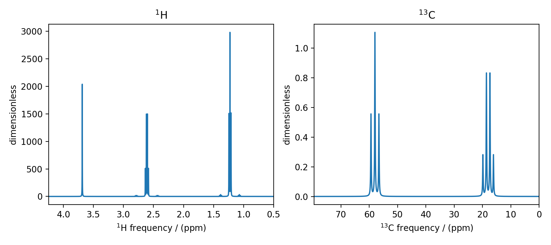
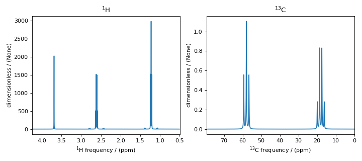
Figure 8 \(^1\text{H}\) and \(^{13}\text{C}\) spectrum of ethanol. Note, the \(^{13}\text{C}\) satellites seen on either side of the peaks near 1.2 ppm and 2.6 ppm in the \(^1\text{H}\) spectrum.

Saving your Work

Saving the Spectra

You can save the spectra in csdf format using the code below.

processed_H_spectrum.save("processed_H_spectrum.csdf")
processed_C_spectrum.save("processed_C_spectrum.csdf")

Saving the SpinSystems

If you want to save the spin systems for use in a different project, you can ask the Simulator instance to export the list of SpinSystem instances to a JSON file with the code below.

sim.export_spin_systems("ethanol.mrsys")

The file ethanol.mrsys holds a JSON representation of the SpinSystem instances. We encourage the convention of using .mrsys extension for this JSON file.

The list of SpinSystem instances can be reloaded back into a Simulator instance by calling load_spin_systems() with the file name of the saved SpinSystem objects, as shown below.

new_sim = Simulator()
new_sim.load_spin_systems("ethanol.mrsys")

Saving the Methods

Similarly, if you want to save the methods for use in another project, you can ask the Simulator instance to export the list of Method instances to a JSON file.

sim.export_methods("H1C13Methods.mrmtd")

As before, the file H1C13Methods.mrmtd holds a JSON representation of the method instances. We encourage the convention of using .mrmtd extension for this JSON file.

The list of Method instances can also be reloaded back into a Simulator instance by calling load_methods() with the file name of the saved Method instances as shown below.

new_sim = Simulator()
new_sim.load_methods("H1C13Methods.mrmtd")

Saving the full Simulation

The Simulation and SignalProcessor instances can also be serialized into JSON files. At some point, however, saving the Python script or Jupyter Notebook with your code will be just as convenient. Nonetheless, you can find additional details on JSON serialization of MRSimulator instances in the MRSimulator I/O section.