Signal Processor¶

After running a simulation, you may need to apply some post-simulation signal processing. For example, you may need to scale the simulated spectrum to match experimental intensities, or you may want to convolve the spectrum with a Lorentzian, Gaussian, or other line-broadening function. For this reason, mrsimulator offers some frequently used NMR signal processing tools within the mrsimulator.signal_processor module.

CSDM object¶

The simulated spectrum is held in a CSDM [1] object, which supports multi-dimensional scientific datasets (NMR, EPR, FTIR, GC, etc.). For more information, see the csdmpy documentation.

`SignalProcessor` class¶

Signal processing is a series of operations sequentially applied to the dataset. In mrsimulator, the SignalProcessor object is used to apply operations. Here we create a new SignalProcessor object

# Import the signal_processor module
from mrsimulator import signal_processor as sp

# Create a new SignalProcessor object
processor = sp.SignalProcessor()

Each signal processor object holds a list of operations under the operations attribute. Below we add operations to apply Gaussian line broadening and a scale factor.

processor.operations = [
    sp.IFFT(),
    sp.apodization.Gaussian(FWHM="50 Hz"),
    sp.FFT(),
    sp.Scale(factor=120),
]

First, an inverse Fourier transform is applied to the dataset, converting it to the time domain. Then, a Gaussian apodization, parameterized using a full-width-at-half-maximum (FWHM) of 50 Hz, is applied. Note, the dimensionality of the FWHM attribute has the inverse dimensionality of the dataset domain. Finally, a forward Fourier transform is applied to the apodized dataset, and all points are scaled up by 120 times.

Note

Convolutions in mrsimulator are performed using the Convolution Theorem. A spectrum is Fourier transformed, and apodizations are performed in the time domain before being transformed back into the frequency domain.

Let’s create a CSDM object and then apply the operations to visualize the results.

import csdmpy as cp
import numpy as np

# Create a CSDM object with delta function at 200 Hz
test_data = np.zeros(500)
test_data[200] = 1
csdm_object = cp.CSDM(
    dependent_variables=[cp.as_dependent_variable(test_data)],
    dimensions=[cp.LinearDimension(count=500, increment="1 Hz")],
)

To apply the previously defined signal processing operations to the above CSDM object, use the apply_operations() method of the SignalProcessor instance as follows

processed_dataset = processor.apply_operations(dataset = csdm_object)

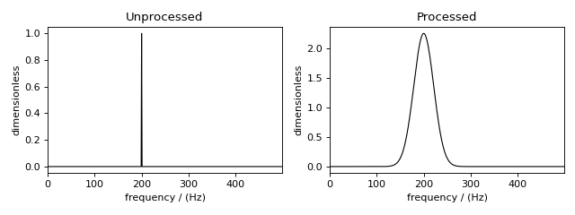
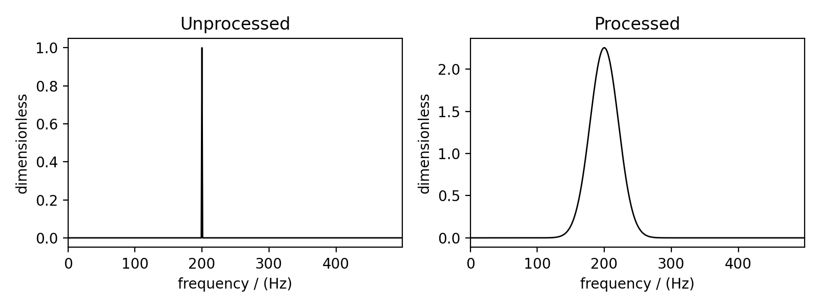
The variable processed_dataset is another CSDM object holding the dataset after the list of operations has been applied to csdm_object. Below is a plot comparing the unprocessed and processed dataset

import matplotlib.pyplot as plt
_, ax = plt.subplots(1, 2, figsize = (8, 3), subplot_kw = {"projection":"csdm"})
ax[0].plot(csdm_object, color="black", linewidth=1)
ax[0].set_title("Unprocessed")
ax[1].plot(processed_dataset.real, color="black", linewidth=1)
ax[1].set_title("Processed")
plt.tight_layout()
plt.show()

(png, hires.png, pdf)

../../_images/signal_processor-5.png — Figure 53 The unprocessed dataset (left) and processed dataset (right) with a Gaussian convolution and scale factor.¶

Applying Operations along a Dimension¶

Multi-dimensional NMR simulations may need different operations applied along different dimensions. Each operation has the attribute dim_index, which is used to apply operations along a certain dimension.

By default, dim_index is None and is applied along the 1st dimension. An integer or list of integers can be passed to dim_index, specifying the dimensions. Below are examples of specifying the dimensions

# Gaussian apodization along the first dimension (default)
sp.apodization.Gaussian(FWHM="10 Hz")

# Constant offset along the second dimension
sp.baseline.ConstantOffset(offset=10, dim_index=1)

# Exponential apodization along the first and third dimensions
sp.apodization.Exponential(FWHM="10 Hz", dim_index=[0, 2])

Applying Apodizations to specific Dependent Variables¶

Each dimension in a simulated spectrum can hold multiple dependent variables (a.k.a. contributions from multiple spin systems). Each spin system may need different convolutions applied to match an experimental spectrum. The Apodization sub-classes have the dv_index attribute, specifying which dependent variable (spin system) to apply the operation on. By default, dv_index is None and will apply the convolution to all dependent variables in a dimension.

Note

The index of a dependent variable (spin system) corresponds to the order of spin systems in the spin_systems list.

processor = sp.SignalProcessor(
    operations=[
        sp.IFFT(),
        sp.apodization.Gaussian(FWHM="25 Hz", dv_index=0),
        sp.apodization.Gaussian(FWHM="70 Hz", dv_index=1),
        sp.IFFT(),
    ]
)

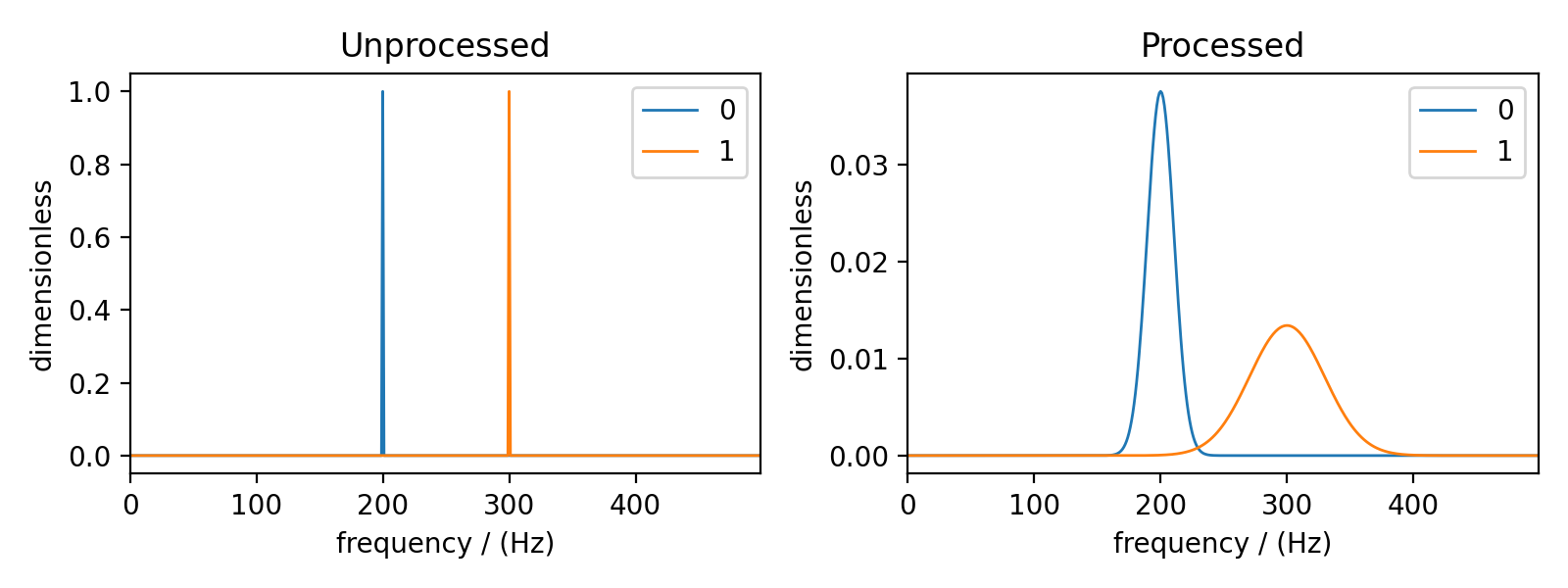
The above list of operations will apply 25 and 70 Hz of Gaussian line broadening to dependent variables at index 0 and 1, respectively.

Let’s add another dependent variable to the previously created CSDM object to target specific dependent variables.

test_data = np.zeros(500)
test_data[300] = 1
csdm_object.add_dependent_variable(cp.as_dependent_variable(test_data))

Now, we again apply the operations with the apply_operations() method. The comparison of the unprocessed and processed dataset is also shown below.

processed_dataset = processor.apply_operations(dataset = csdm_object)

Below is a plot of the dataset before and after applying the operations

_, ax = plt.subplots(1, 2, figsize=(8, 3), subplot_kw={"projection":"csdm"})
ax[0].plot(csdm_object, linewidth=1)
ax[0].set_title("Unprocessed")
ax[1].plot(processed_dataset.real, linewidth=1)
ax[1].set_title("Processed")
plt.tight_layout()
plt.show()

(png, hires.png, pdf)

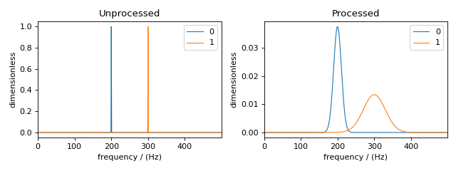
../../_images/signal_processor-10.png — Figure 55 The unprocessed dataset (left) and the processed dataset (right) with convolutions applied to different dependent variables.¶

Signal Processor¶

CSDM object¶