Simulator

Overview

The Simulator is the top-level class in MRSimulator. The two main attributes of the Simulator class are spin_systems and methods, which hold a list of SpinSystem and Method instances, respectively. In addition, the simulator class also contains a config attribute, which holds a ConfigSimulator instance. The ConfigSimulator class configures the simulation properties, which may be useful in optimizing simulations.

In this section, you will learn about the ConfigSimulator attributes. For simplicity, the following code pre-defines the plot function to use further in this document.

import matplotlib.pyplot as plt

# function to render figures.
def plot(csdm_instance, labels):
    csdm_instance = csdm_instance if isinstance(csdm_instance, list) else [csdm_instance]
    _, ax = plt.subplots(1, len(csdm_instance), figsize=(8, 3), subplot_kw={"projection": "csdm"})
    ax = [ax] if len(csdm_instance) == 1 else ax
    for i, obj in enumerate(csdm_instance):
        ax[i].plot(obj.real, linewidth=1.5)
        ax[i].set_title(labels[i])
        ax[i].invert_xaxis()
    plt.tight_layout()
    plt.show()

ConfigSimulator

In mrsimulator, the default configuration settings apply to a wide range of simulations, including static, magic angle spinning (MAS), and variable angle spinning (VAS) spectra. In certain situations, however, the default settings are insufficient to represent the spectrum accurately. In this section, we use the simulator setup code below to illustrate some of these issues.

from mrsimulator import Site, Simulator, SpinSystem
from mrsimulator.spin_system.tensors import SymmetricTensor
from mrsimulator.method import SpectralDimension
from mrsimulator.method.lib import BlochDecaySpectrum

# Setup the spin system and method instances
Si29_site = Site(
    isotope="29Si",
    shielding_symmetric=SymmetricTensor(
        zeta=100,  # in ppm
        eta=0.2,
        alpha=1.563,  # in rads
        beta=1.2131,  # in rads
        gamma=2.132,  # in rads
    )
)
system = SpinSystem(sites=[Si29_site])

method = BlochDecaySpectrum(
    channels=["29Si"],
    rotor_frequency=0,  # in Hz
    spectral_dimensions=[SpectralDimension(count=1024, spectral_width=25000)]
)

# Create the Simulator instance
sim = Simulator(spin_systems=[system], methods=[method])

Here, sim is a Simulator instance that holds one spin system and one method. See Spin System and Method documentation for more information on the respective classes.

---

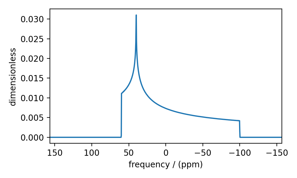
Integration Volume

The attribute integration_volume is an enumeration of string literals, octant, hemisphere, and sphere. The integration volume refers to the volume of a unit sphere over which the integrated NMR frequencies are evaluated. The default value is octant, i.e., the spectrum comprises integrated frequencies from the positive octant of a unit sphere. MRSimulator can exploit the problem’s orientational symmetry, thus optimizing the simulation by performing a partial integration.

To learn more about the orientational symmetries, refer to Eden et al. [1]

Consider the \(^{29}\text{Si}\) site, Si29_site, from the above setup. This site has a symmetric shielding tensor with zeta and eta as 100 ppm and 0.2, respectively. With only zeta and eta (and zero Euler angles), we could exploit the symmetry of the problem and evaluate the frequency integral over the octant, equivalent to integration over a sphere. The non-zero Euler angles for this tensor break the symmetry, and integration over the octant will no longer be accurate. To fix this inaccuracy, set the integration volume to hemisphere and re-simulate.

sim.run()
inaccurate_sim = sim.methods[0].simulation

# set integration volume to hemisphere
sim.config.integration_volume = "hemisphere"
sim.run()
accurate_sim = sim.methods[0].simulation

plot([inaccurate_sim, accurate_sim], labels=["octant", "hemisphere"])

(png, hires.png, pdf)

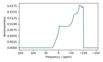
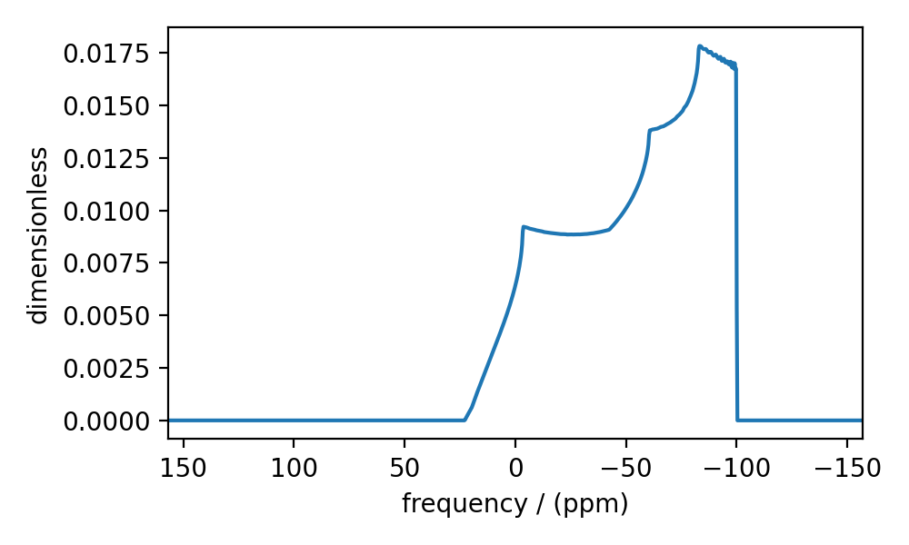
Figure 33 (left) Inaccurate simulation resulting from integrating over an octant when the spin system contains non-zero Euler angles. (right) Accurate CSA spectrum resulting from the frequency contributions evaluated over the top hemisphere.

Integration Density

The attribute integration_density controls the number of orientations sampled over the given volume. The resulting spectrum is the integrated NMR resonance frequency evaluated over these orientations. The total number of orientations, \(\Theta_\text{count}\), is

(40)\[\Theta_\text{count} = M (n + 1)(n + 2)/2\]

where \(M\) is the number of octants and \(n\) is the value of this attribute. The number of octants is the value from the integration_volume attribute. The default value of this attribute, 70, produces 2556 orientations at which the NMR frequency contributions are evaluated.

sim.config.integration_density = 10
sim.run()
low_density_sim = sim.methods[0].simulation

# increase the sampling density
sim.config.integration_density = 100
sim.run()
high_density_sim = sim.methods[0].simulation

plot([low_density_sim, high_density_sim], labels=["low density", "high density"])

(png, hires.png, pdf)

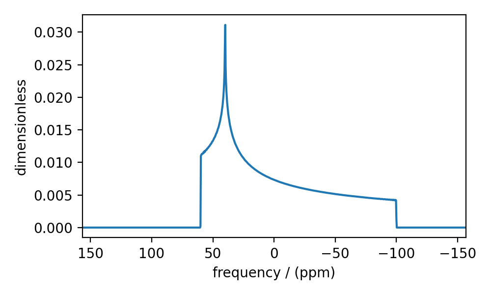
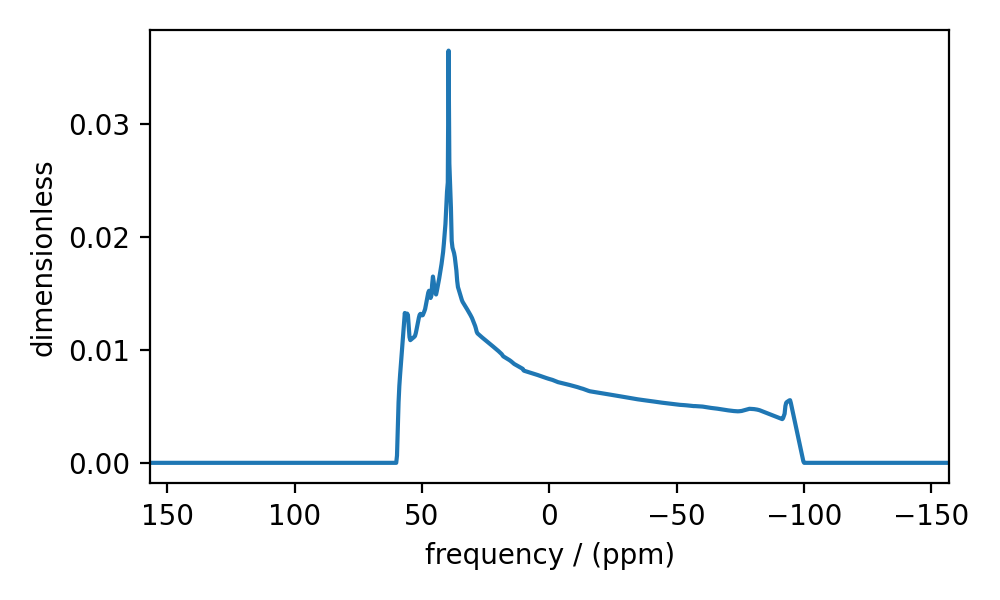
Figure 35 (left) Low-quality simulation from reduced integration density (=10). (right) High-quality simulation from increased integration density (=100).

Decreasing the integration density may decrease the simulation time for computationally intensive simulations but at the cost of spectrum quality. Generally, use a higher integration density for a high-resolution spectrum (i.e., a high-resolution sampling grid). For a low-resolution sampling grid, the spectrum may converge with a lower integration density.

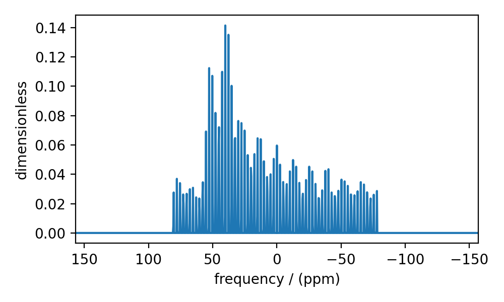
Number of Sidebands

The number_of_sidebands attribute determines the number of sidebands evaluated in the simulation. The default value is 64 which is sufficient for most cases.

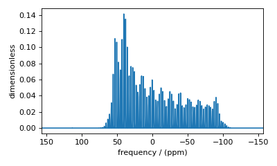
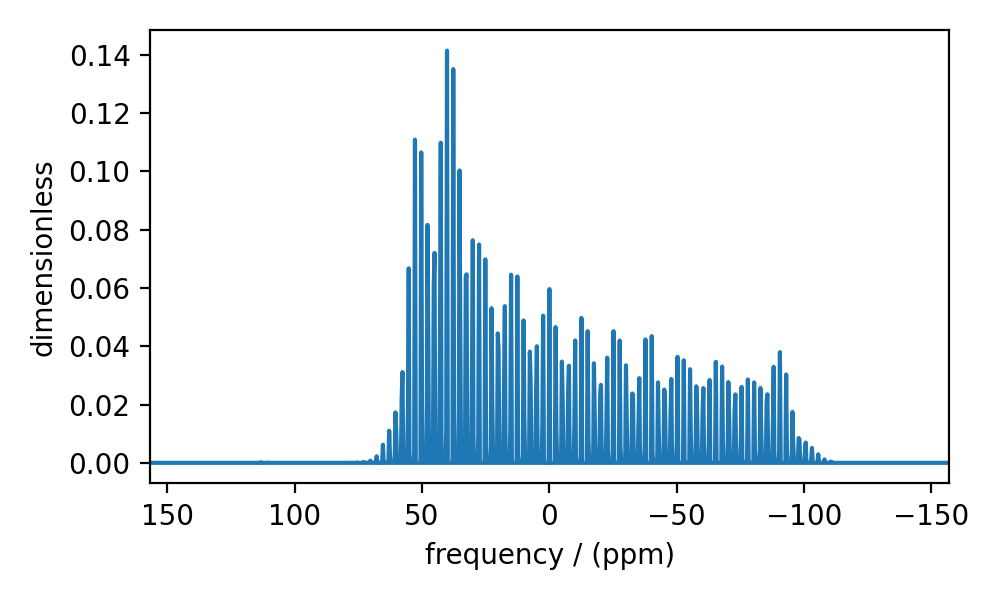
In certain circumstances, especially when the anisotropy is large or the rotor spin frequency is low, 64 sidebands might not be sufficient. For the figure on the left, the spinning sideband amplitude patterns abruptly terminate at the edges. This inaccuracy arises from evaluating a small number of sidebands relative to the size of anisotropy. Increasing the number of sidebands will resolve this issue (see the figure on the right).

sim.methods[0] = BlochDecaySpectrum(
    channels=["29Si"],
    rotor_frequency=200,
    spectral_dimensions=[SpectralDimension(count=1024, spectral_width=25000)],
)
sim.run()
low_n_sidebands = sim.methods[0].simulation

# increase the number of sidebands
sim.config.number_of_sidebands = 90
sim.run()
high_n_sidebands = sim.methods[0].simulation

plot([low_n_sidebands, high_n_sidebands], labels=["low #sidebands", "high #sidebands"])

(png, hires.png, pdf)

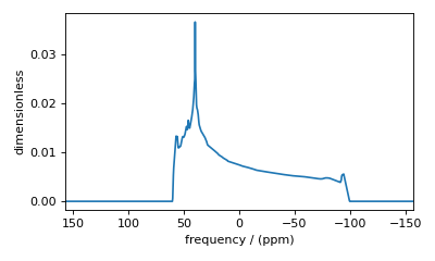
Figure 37 (left) Inaccurate sideband simulation resulting from computing a low number of sidebands. (right) Accurate sideband simulation after increasing the number of sidebands.

Conversely, 64 sidebands might be excessive, in which case reducing the number of sidebands may significantly improve simulation performance, especially in iterative algorithms, such as the least-squares minimization.

Custom Sampling

The attribute custom_sampling holds a CustomSampling instance that overrides the default ASG orientation sampling, that is, the config attributes integration_density and integration_volume are ignored, allowing the users to specify a custom spatial sampling for spectral integration.

The CustomSampling class instance includes attributes, alpha, beta, and weight which hold a 1D array of \(\alpha\) and \(\beta\) Euler angles (in radians) along with their respective weights. When specified, Mrsimulator uses the user-provided Euler angles for spectral integration. Mrsimulator additionally supports triangle interpolation for 1D and 2D spectral lineshape interpolation. To invoke triangle interpolation, the users may additionally provide a list of triangle vertex indexes as an Nx3 matrix, where N is the number of triangles forming the surface of octant, hemisphere, or sphere, using the vertex_indexes attribute. Note, that when specifying the vertex indexes, the indexing in Python starts with 0.

from mrsimulator.simulator.config import CustomSampling

sim.methods[0] = BlochDecaySpectrum(
    channels=["29Si"],
    rotor_frequency=2000,
    spectral_dimensions=[SpectralDimension(count=600, spectral_width=30000)],
)
sim.config.integration_volume = "hemisphere"
sim.run()
asg_sim = sim.methods[0].simulation

# update the orientation averaging to custom sampling
# load angles from the file
alpha, beta, weight = np.loadtxt('zcw_h_987.bz2', unpack=True)
# create the CustomSampling instance and assign to the config
my_sampling = CustomSampling(
    alpha=alpha.copy(),
    beta=beta.copy(),
    weight=weight.copy()
)
sim.config.custom_sampling = my_sampling
sim.run()
zcw_sim = sim.methods[0].simulation

plot([asg_sim, zcw_sim], labels=["ASG sampling", "ZCW sampling"])

(png, hires.png, pdf)

Figure 39 (left) Simulation using the Mrsimulator default ASG sampling. (right) Simulation using a user-defined custom ZCW sampling.

Number of gamma angles

The number_of_gamma_angles attribute determines the extent of gamma averaging in the simulation. The gamma angles range from \(0\) to \(2\pi\). The default value is 1, corresponding to \(\gamma=0\).

In most static powder simulations, you can get by with one gamma angle (default) by appropriately setting the rotor_angle=0. When evaluating a static powder simulation for a non-zero rotor_angle, use a large number of gamma angles for the simulation to converge. To resolve this, increase the number of gamma angles.

from mrsimulator.method import Method
from mrsimulator.method.event import SpectralEvent, RotationEvent

site = Site(isotope="29Si", shielding_symmetric={"zeta": 100, "eta": 0.2})
spin_system = SpinSystem(sites=[site])

solid_echo = Method(
    channels=["29Si"],
    rotor_frequency=0,  # in Hz
    rotor_angle=54.734 * np.pi / 180,  # in rads
    spectral_dimensions=[
        SpectralDimension(
            count=1024,
            spectral_width=25000,
            events=[
                SpectralEvent(fraction=0.5, transition_queries=[{"ch1": {"P": [-1]}}]),
                RotationEvent(ch1={"angle": np.pi / 2}),
                SpectralEvent(fraction=0.5, transition_queries=[{"ch1": {"P": [-1]}}]),
            ]
    )],
)

sim = Simulator(spin_systems=[spin_system], methods=[solid_echo])
sim.run()
one_gamma_angle = sim.methods[0].simulation

# increase the number of gamma angles
sim.config.number_of_gamma_angles=1000
sim.run()
n_gamma_angle = sim.methods[0].simulation

plot([one_gamma_angle, n_gamma_angle], labels=["Default 1 gamma angle", "1000 gamma angles"])

(png, hires.png, pdf)

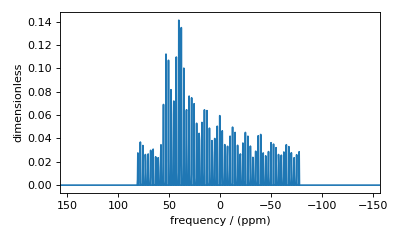
Figure 41 (left) Incorrect simulation from an insufficient number of gamma angle averaging. (right) Accurate simulation from a sufficiently large number of gamma angle averaging.

Decompose Spectrum

The attribute decompose_spectrum is an enumeration with two string literals, none and spin_system. The default value is none.

If the value is none (default), the resulting simulation is a single spectrum where the frequency contributions from all the spin systems are co-added. Consider the example below. When the value of decompose_spectrum is spin_system, the resulting simulation is a series of subspectra corresponding to individual spin systems. The number of subspectra equals the number of spin systems within the Simulator instance. Consider the following example with two spin systems simulated with decompose_spectrum attribute set to default none and spin_system.

# Create two distinct sites
site_A = Site(
    isotope="1H",
    shielding_symmetric=SymmetricTensor(zeta=5, eta=0.1),
)
site_B = Site(
    isotope="1H",
    shielding_symmetric=SymmetricTensor(zeta=-2, eta=0.83),
)

# Create two single site spin systems
sys_A = SpinSystem(sites=[site_A], name="System A")
sys_B = SpinSystem(sites=[site_B], name="System B")

# Create a method representing a simple 1-pulse acquire experiment
method = BlochDecaySpectrum(
    channels=["1H"], spectral_dimensions=[SpectralDimension(count=1024, spectral_width=10000)]
)

# Create Simulator instance, simulate, and plot
sim = Simulator(spin_systems=[sys_A, sys_B], methods=[method])
sim.run()
averaged_sim = sim.methods[0].simulation

# sim already has the two spin systems and method; no need to reconstruct
sim.config.decompose_spectrum = "spin_system"
sim.run()
decomposed_dim = sim.methods[0].simulation

plot([averaged_sim, decomposed_dim], labels=["Averaged", "Decomposed"])

(png, hires.png, pdf)

Figure 43 (left) The frequency contributions from individual spin systems are combined into one spectrum. (right) Each spin system’s frequency contributions are held in separate spectra.

Isotropic interpolation

The attribute isotropic_interpolation is an enumeration with two string literals, linear and gaussian. The default value is linear.

The value specifies the interpolation scheme used in binning purely isotropic spectrum.

Attribute Summaries

Table 13 The attributes of a Simulator instance

Attribute Name	Type	Description
spin_systems	list	An optional list of SpinSystem instances.
methods	list	An optional list of Method instances.
config	dict or ConfigSimulator	An optional ConfigSimulator instance or its dictionary representation.

Table 14 The attributes of the Simulator class

Attribute Name	Type	Description
number_of_sidebands	int	An optional integer greater than zero specifying the number of sidebands to simulate. The default is 64 sidebands.
integration_volume	str	An optional string representing the fraction of a unit sphere used in the integrated NMR frequency spectra. The allowed strings are octant, hemisphere, and sphere. The default is octant.
integration_density	int	An optional integer greater than zero specifying the number of orientations sampled over the given volume according to the equation \(\Theta_\text{count} = M (n + 1)(n + 2)/2\), where \(M\) is the number of octants. The default value is 70.
decompose_spectrum	str	An optional string specifying the spectral decomposition type. The allowed strings are none and spin_system. The value of none produces one spectrum averaged over all spin systems, while spin_system produces a series of subspectra corresponding to individual spin systems. The default is none.
isotropic_interpolation	str	An optional string specifying the interpolation scheme used in binning purely isotropic subspectra. The allowed strings are linear and gaussian. The default is linear.

---

[1]

Edén, M. and Levitt, M. H. Computation of orientational averages in solid-state nmr by gaussian spherical quadrature. J. Mag. Res., 132, 2, 220-239, 1998. doi:10.1006/jmre.1998.1427.