Getting Started¶

In mrsimulator, the user initializes objects from mrsimulator classes; The three main classes we will use in this example are: Spin System, Method, and Simulator.

SpinSystem defines the spin system and its tensor parameters used to generate a particular subspectrum, and Method defines the behavior and parameters for the particular NMR measurement to be simulated. A list of Method and SpinSystem objects are used to initialize a Simulator object, which is then used to generate the corresponding NMR spectra—returned as a CSDM object in each Method object. For more information on the CSDM (Core Scientific Dataset Model), see the csdmpy documentation. There is an additional class, Signal Processor, for applying various post-simulation signal processing operations to CSDM dataset objects.

All objects in mrsimulator can be serialized. We adopt the Javascript Object Notation (JSON) as the file-serialization format for the model because it is human-readable if properly organized and easily integrable with numerous programming languages and related software packages. It is also the preferred serialization for data exchange in web-based applications.

Here, we have put together a tutorial which introduces the key objects in a typical mrsimulator workflow. See the User Documentation section for more detailed documentation on the usage of mrsimulator classes. Also, check out our Simulation Gallery and Fitting (Least Squares) Gallery.

SpinSystem¶

An NMR spin system is an isolated system of sites (spins) and couplings. Spin systems can include as many sites and couplings as necessary to model a sample. For this introductory example, you will create a coupled \(^1\text{H}\) - \(^{13}\text{C}\) spin system. Use the code below to construct two Site objects for the \(^1\text{H}\) and \(^{13}\text{C}\) sites.

# Import the Site and SymmetricTensor classes
from mrsimulator import Site
from mrsimulator.spin_system.tensors import SymmetricTensor

# Create the Site objects
H_site = Site(isotope="1H")
C_site = Site(
    isotope="13C",
    isotropic_chemical_shift=100.0,  # in ppm
    shielding_symmetric=SymmetricTensor(
        zeta=70.0,  # in ppm
        eta=0.5,
    ),
)
my_sites = [H_site, C_site]

Note that isotopes in mrsimulator are specified with a string that starts with the isotope’s mass number followed by its element symbol.

In the code above, you created two Site objects in the variables H_site and C_site. The H_site variable represents a proton site with a (default) chemical shift of zero. The C_site variable represents a carbon-13 site with a chemical shift of 100 ppm and a shielding component represented by a SymmetricTensor object. We parametrize tensors using the Haeberlen convention. All spin interaction parameters, e.g., isotropic chemical shift and other coupling parameters, are initialized to zero by default. Additionally, the default Site isotope is 1H.

At the end of the code above, you placed H_site and C_site into a Python list named my_sites. The order of Sites in this list is important, as the indexes of Sites in this list are used when specifying couplings between sites. Note that indexes in Python start at zero.

Using the code below, define a dipolar coupling between H_site and C_site by creating a Coupling object.

# Import the Coupling class
from mrsimulator import Coupling

# Create the Coupling object
coupling = Coupling(
    site_index=[0, 1],
    dipolar=SymmetricTensor(D=-2e4),  # in Hz
)

The two sites involved in the Coupling are identified by their indexes in the list variable site_index.

Now you have all the pieces needed to create the spin system using the code below.

# Import the SpinSystem class
from mrsimulator import SpinSystem

# Create the SpinSystem object
spin_system = SpinSystem(
    sites = my_sites,
    couplings=[coupling],
)

That’s it! You have created a spin system whose spectrum is ready to be simulated. If you had wanted to create an uncoupled spin system, simply omit the couplings attribute.

Method¶

A Method object in mrsimulator describes an NMR method. For this introduction, you can use the pre-defined method BlochDecaySpectrum. This method simulations the spectrum obtained from the Fourier transform of a Bloch decay signal, i.e., one-pulse and acquire. You can use the code below to create the Method object initialized with attributes whose names should be relatively familiar to an NMR spectroscopist.

# Import the BlochDecaySpectrum class
from mrsimulator.method.lib import BlochDecaySpectrum
from mrsimulator.method import SpectralDimension

# Create a BlochDecaySpectrum object
method = BlochDecaySpectrum(
    channels=["13C"],
    magnetic_flux_density=9.4,  # in T
    rotor_angle=54.735 * 3.14159 / 180,  # in rad (magic angle)
    rotor_frequency=3000,  # in Hz
    spectral_dimensions=[
        SpectralDimension(
            count=2048,
            spectral_width=80e3,  # in Hz
            reference_offset=6e3,  # in Hz
            label=r"$^{13}$C resonances",
        )
    ],
)

The channel attribute holds a list of isotope strings. In the BlochDecaySpectrum method, however, only the first isotope in the list, i.e., \(^{13}\text{C}\), is used to simulate the spectrum. The BlochDecaySpectrum method has one spectral dimension. In this example, that spectral dimension has 2048 points, spanning 80 kHz with a reference offset of 6 kHz.

Next, you will bring the SpinSystem and Method objects together and create a Simulator object that will simulate the spectrum.

Simulator¶

At the heart of mrsimulator is the Simulator object, which calculates the NMR spectrum. Mrsimulator performs all calculations in the frequency domain, and all resonance frequencies are calculated in the weakly-coupled (Zeeman) basis for the spin system.

In the code below, you create a Simulator object, initialized with your previously defined spin system and method, and then call run() on your Simulator object.

# Import the Simulator class
from mrsimulator import Simulator

# Create a Simulator object
sim = Simulator(spin_systems=[spin_system], methods=[method])
sim.run()

The simulated spectrum is stored as a CSDM object in the Method object at sim.methods[0].simulation. To match an experimental MAS spectrum, however, you still need to add some line broadening to the simulated spectrum. For this, you can use the Signal Processor object described in the next section.

SignalProcessor¶

A Signal Processor object holds a list of operations applied sequentially to a dataset. For a comprehensive list of operations and further details on using the SignalProcessor object, consult the Signal Processor documentation.

Use the code below to create a SignalProcessor object that performs a convolution of the simulated spectrum with a Lorentzian distribution having a full-width-half-maximum of 200 Hz. This is done with three operations: the first operation applies an inverse fast Fourier transform of the spectrum into the time domain, the second operation applies a time-domain apodization with an exponential decay, and the third operation applies a fast Fourier transform back into the frequency domain.

from mrsimulator import signal_processor as sp

# Create the SignalProcessor object
processor = sp.SignalProcessor(
    operations=[
        sp.IFFT(),
        sp.apodization.Exponential(FWHM="200 Hz"),
        sp.FFT(),
    ]
)

# Apply the processor to the simulation dataset
processed_simulation = processor.apply_operations(dataset=sim.methods[0].simulation)

PyPlot¶

You can use Matplotlib’s PyPlot module to plot your simulations. To aid in plotting CSDM objects with PyPlot, csdmpy provides a custom CSDM dataset plot axes. To use it, simply pass projection="csdm" when instantiating an Axes instance. Below is code using the PyPlot module which will generate a plot and a pdf file of the simulated spectrum:

Note

To use the custom CSDM axes with projection="csdm", the csdmpy library needs imported.

import matplotlib.pyplot as plt

plt.rcParams['pdf.fonttype'] = 42   # For using plots in Illustrator
plt.figure(figsize=(5, 3))  # set the figure size
ax = plt.subplot(projection="csdm")
ax.plot(processed_simulation.real)
ax.invert_xaxis()  # reverse x-axis
plt.tight_layout()
plt.savefig("spectrum.pdf")
plt.show()

(png, hires.png, pdf)

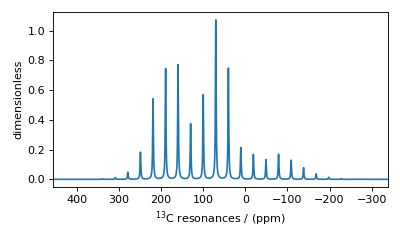
../_images/getting_started-7.png — Figure 5 A simulated \(^{13}\text{C}\) MAS spectrum.¶

The plt.savefig("spectrum.pdf") line creates a pdf file that can be edited in a vector graphics editor such as Adobe Illustrator. We encourage you to work through the PyPlot basic usage tutorial to understand its methods and learn how to further customize your plots.

CSDM¶

Mrsimulator is designed to be part of a larger data workflow involving other software packages. For this larger context, mrsimulator uses the Core Scientific Dataset Model (CSDM) for importing and exporting your datasets. CSDM is a lightweight, portable, human-readable, and versatile standard for intra- and interdisciplinary exchange of scientific datasets. The model supports multi-dimensional datasets with a multi-component dependent variable discretely sampled at unique points in a multi-dimensional independent variable space. It can also hold correlated datasets assuming the different physical quantities (dependent variables) are sampled on the same orthogonal grid of independent variables. It can even handle datasets with non-uniform sampling on a grid. The CSDM can also serve as a re-usable building block in developing more sophisticated portable scientific dataset file standards.

Mrsimulator also uses CSDM internally as its object model for simulated and experimental datasets. Any CSDM object in mrsimulator can be serialized as a JavaScript Object Notation (JSON) file using its save() method. For example, the simulation after the signal processing step above is saved as a csdf file as shown below.

processed_simulation.save("processed_simulation.csdf")

For more information on the CSDM file formats, see the csdmpy documentation.