Least-Squares Fitting Example¶

MRSimulator can interact with various Python data science packages. One such package, LMFIT, can be used to perform non-linear least-squares analysis of experimental NMR spectra.

Here, we illustrate the use of the MRSimulator instances to

import and prepare an experimental dataset for the least-squares analysis,
create a fitting model using Simulator and SignalProcessor instances,
use the fitting model to perform a least-squares analysis,
extract the model parameters with uncertainties and
plot the experimental spectrum along with the best-fit simulation and residuals.

Import Experimental Dataset¶

In this example, you will apply the least-squares fitting procedure to a $^{27}\text{Al}$ magic-angle spinning spectrum of $\text{Al(acac)$_3$}$ measured with whole echo acquisition.

You will begin by importing an experimental dataset measured on a 9.4 T Bruker AVANCE III HD NMR spectrometer into the script. Bruker datasets are saved in folders with a number as the folder name. In this case, that folder has been transferred from the spectrometer and renamed “Al_acac”.

Download experimental dataset¶

For our purposes, the folder was also compressed into a zip archive and uploaded to an internet-accessible server. You can use the code block below to download the zip archive from the server and unzip it into the originally named folder.

import requests
import zipfile
from io import BytesIO

file_ = "https://ssnmr.org/sites/default/files/mrsimulator/Al_acac3_0.zip"
request = requests.get(file_)
z = zipfile.ZipFile(BytesIO(request.content))
z.extractall("Al_acac")

Convert experimental dataset to CSDM¶

Now that the Bruker dataset folder is accessible to your Python code, you can use the Python package nmrglue to convert the dataset into a CSDM object.

import nmrglue as ng

# initialize nmrglue converter object
converter = ng.convert.converter()

# read in the bruker dataset file
dic, data = ng.bruker.read("Al_acac")
converter.from_bruker(dic, data)

# convert to CSDM format
csdm_ds = converter.to_csdm()

Once imported, it is necessary to update a few attributes of the CSDM instance in the code below.

# set origin offset to primary reference
csdm_ds.dimensions[0].reciprocal.origin_offset = "104.38311571 MHz"

# and set coordinates offset to carrier frequency
csdm_ds.dimensions[0].reciprocal.coordinates_offset = "-538.05 Hz"

# set time origin to echo top
csdm_ds.dimensions[0].coordinates_offset = "-8.16 ms"

Specifically, the reciprocal.origin_offset attribute of is set to 104.38311571 MHz, the $^{27}\text{Al}$ primary reference resonance frequency measured on this spectrometer using a 1.1 mol/kg solution of $\text{Al(NO$_3$)$_3$}$ as an external standard. Additionally, the reciprocal.coordinates_offset attribute is set to the offset between the primary reference resonance frequency and the spectrometer carrier frequency. In principle, these two steps should not be necessary as these two attributes should have been set correctly when the Bruker dataset is imported. However, it is not uncommon that were not set correctly during the data acquisition. Thus, it is always a good idea to check and adjust these values as needed.

Additionally, since this signal is acquired with a Hahn-echo sequence, with acquisition beginning immediately after the 180 deg. pulse, the coordinates_offset needs to be adjusted to place the time origin at the top of the echo. This should be the time between the centers of the two pulses. There are, however, some additional receiver delays before the signal acquisition begins, and those times, which are among the pulse sequence parameters, need to be subtracted from the inter-pulse spacing. For this measurement, we have predetermined the echo top position to be 8.16 ms. Thus, we set the coordinates_offset attribute to -8.16 ms.

With the dataset converted into a CSDM instance, plot the dataset to make sure that you imported it correctly.

import matplotlib.pyplot as plt

plt.figure(figsize=(5, 3))  # set the figure size
ax = plt.subplot(projection="csdm")
ax.plot(csdm_ds.real, label="real")
ax.plot(csdm_ds.imag, label="imag")
plt.tight_layout()
plt.grid()
plt.legend()
plt.show()

(png, hires.png, pdf)

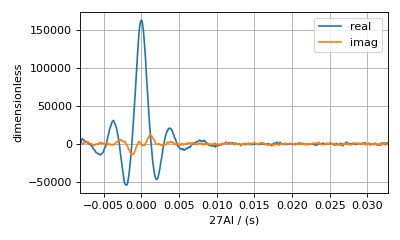
This is the raw time-domain dataset, acquired using whole-echo acquisition. The blue and orange lines are the real and imaginary parts of the complex time-domain signal. If you’re working with your own experimental dataset and have already processed it into the frequency domain, then you can skip the next few steps and proceed to the Measure Noise section.

Process Experimental Dataset¶

Proceeding from here, you’ll need to transform this dataset into the frequency domain for the least-squares analysis. Before applying the Fourier transform, however, two things need to be adjusted.

First, you need to phase correct the time domain so that the maximum echo amplitude is in the real part of the signal. For this operation, you can use numpy abs () to take the absolute value of each complex signal amplitude, and numpy argmax () to find the time index where the absolute value of the signal is at a maximum. Then use the signal phase at that time index to place the maximum amplitude into the real part of the time domain signal.

These steps are performed by the code below.

import numpy as np

# Phase echo top, putting maximum amplitude into real part
index = np.argmax(np.abs(csdm_ds.dependent_variables[0].components[0]))
angle = np.angle(csdm_ds.dependent_variables[0].components[0][index])
phased_ds = csdm_ds * np.exp(-1j * angle)

plt.figure(figsize=(5, 3))  # set the figure size
ax = plt.subplot(projection="csdm")
ax.plot(phased_ds.real, label="real")
ax.plot(phased_ds.imag, label="imag")
plt.tight_layout()
plt.grid()
plt.legend()
plt.show()

(png, hires.png, pdf)

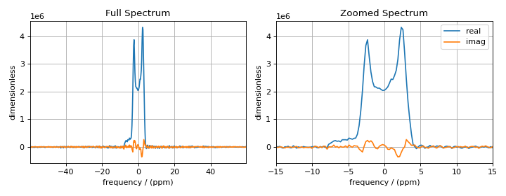
Here, you see that the echo top has been phased so that the maximum amplitude is in the real (blue) part and that the echo top occurs at the time origin. Notice that the echo has a slight asymmetry about the time origin after it has been phased. The first half of the echo has a slightly stronger amplitude than the last half. This asymmetry is due to an additional dephasing caused by homonuclear dipolar couplings among the $^{27}\text{Al}$ nuclei. It may have been possible to remove or minimize the effects of these dipolar couplings using a higher MAS rate. Nonetheless, you can still proceed in this analysis and, as you will see later, can model this additional decay with an ad-hoc Gaussian convolution of the spectrum.

Next, a Fourier transform operation is applied to the CSDM dataset using the .fft() method of the CSDM class, as shown in the code below. Note that with a correctly set time origin, the .fft() method automatically applies the appropriate first-order phase correction to the spectrum after performing the fast Fourier transform. After performing the Fourier transform, convert the coordinate units of the CSDM dimension from frequency to a frequency ratio using the to() method of the Dimension object.

exp_spectrum = phased_ds.fft()
exp_spectrum.dimensions[0].to("ppm", "nmr_frequency_ratio")

fig, ax = plt.subplots(1, 2, figsize=(9, 3.5), subplot_kw={"projection": "csdm"})
ax[0].plot(exp_spectrum.real)
ax[0].plot(exp_spectrum.imag)
ax[0].set_title("Full Spectrum")
ax[0].grid()
ax[1].plot(exp_spectrum.real, label="real")
ax[1].plot(exp_spectrum.imag, label="imag")
ax[1].set_title("Zoomed Spectrum")
ax[1].set_xlim(-20, 10)
ax[1].grid()
plt.tight_layout()
plt.legend()
plt.show()

(png, hires.png, pdf)

Measure Noise¶

Now that you have an adequately phased frequency domain dataset, you’ll need to take the real part of the spectrum for the rest of the analysis, i.e., remove the imaginary part.

The least-squares analysis also needs the standard deviation of the noise in the spectrum. We can obtain that from the spectrum regions below -20 ppm or above 20 ppm, where there is no signal amplitude. To accomplish this, you can use numpy where(). It evaluates a condition for each item in the list and returns the indexes for those items where the condition is true. With the indexes returned by where(), you can calculate the standard deviation of the noise region with numpy std().

# Use only the real part of the spectrum
exp_spectrum = exp_spectrum.real

# Use region below -20 ppm to calculate the noise standard deviation
loc = np.where(exp_spectrum.dimensions[0].coordinates < -20e-6)
sigma = exp_spectrum[loc].std()

You can now move to the next step and create the fitting model.

Create Fitting Model¶

To create a proper fitting model, you’ll need more information about the nuclei being observed, the material’s phase and some idea about the local structure around the atoms holding the observed nuclei. In this example, you know that you are working with $^{27}\text{Al}$, a quadrupolar nucleus with a half-integer spin of 5/2, and that the material, $\text{Al(acac)$_3$}$, is a solid polycrystalline sample. The symmetry of the first-coordination sphere around aluminum is likely low enough to generate a large electric field gradient, and hence a sizeable quadrupolar coupling constant for $^{27}\text{Al}$. These details are usually sorted out before the NMR measurement and used to choose the appropriate NMR methods for the sample. In this example, the measurement was performed under magic-angle spinning at a rotation rate of 12.5 kHz. Due to the expected large quadrupolar coupling, relatively low power rf pulses were used to excite only the central $m = \tfrac{1}{2}\rightarrow-\tfrac{1}{2}$ transition of $^{27}\text{Al}$. The central transition is much narrower and more easily detected than the other transitions. Armed with this understanding of the sample and method, you can proceed to create the fitting model.

To build a spin system, you must know how many magnetically inequivalent nuclei are in the sample and whether couplings are between them. Inspection of the spectrum reveals an anisotropic lineshape that appears to be characteristic of the second-order MAS lineshape of a single site. Knowing this requires that you are already familiar with such lineshapes (MRSimulator can help with that!). One might also hypothesize that there may be other sites with lower intensity present in the spectrum, or perhaps the spectrum, as noted earlier, is from a distribution of $^{27}\text{Al}$ sites with very similar efg tensor parameters and dipolar couplings among them. These are all valid hypotheses and could be used to create more elaborate and perhaps even more realistic spin system models. You can now choose the simplest spin system model with a single $^{27}\text{Al}$ site, as shown in the code below.

from mrsimulator import Site, SpinSystem, Simulator

site = Site(
    isotope="27Al",
    isotropic_chemical_shift=0,
    quadrupolar={"Cq": 3e6, "eta": 0.0},
)
sys = SpinSystem(sites=[site])

The tensor parameters above are an educated guess for the tensor parameters, which can be iteratively refined using the code that follows.

Next, we create the Method instance to model the experimental method used to acquire the spectrum. Choose the BlochDecayCTSpectrum() method since the measurement is designed to excite only the central transition of the $^{27}\text{Al}$ nuclei. From the CSDM instance holding the experimental spectrum, i.e., exp_spectrum, you can extract the relevant parameters for the spectral_dimensions attribute of the BlochDecayCTSpectrum method using the fitting utility function get_spectral_dimensions(). The experimental measurement parameters associated with the method attributes magnetic_flux_density and rotor_frequency are also used in creating this BlochDecayCTSpectrum method. Finally, the Method class has the experiment attribute used to hold the experimental spectrum that is to be modeled with the Method class.

from mrsimulator.method.lib import BlochDecayCTSpectrum
from mrsimulator.utils import get_spectral_dimensions
from mrsimulator.spin_system.isotope import Isotope

spectral_dims = get_spectral_dimensions(exp_spectrum)

Al27 = Isotope(symbol="27Al")
origin_offset = spectral_dims[0]["origin_offset"]
B0 = Al27.ref_freq_to_B0(origin_offset)

MAS = BlochDecayCTSpectrum(
    channels=["27Al"],
    magnetic_flux_density=B0,  # in T
    rotor_frequency=12500,  # in Hz
    spectral_dimensions=spectral_dims,
    experiment=exp_spectrum,  # add the measurement to the method.
)

Create the simulator instance initialized with the SpinSystem and Method instances and run.

sim = Simulator(spin_systems=[sys], methods=[MAS])
sim.run()

Next, two convolutions are needed to model the acquired spectrum correctly: a step function to account for the truncation of the echo signal at -8.16 ms, and a Gaussian line shape convolution as an ad-hoc modeling of other residual line broadenings, including transverse relaxation.

Additionally, you must scale the simulation in intensity to match the experimental spectrum. You may have noticed in earlier plots that the vertical axis of the experimental spectrum plot was on the order of 1e6. Use numpy max() to get the highest amplitude, set that as the factor as a Scale operation in the SignalProcessor.

from mrsimulator import signal_processor as sp

# Post Simulation Processing
# --------------------------
relative_intensity_factor = exp_spectrum.max() / sim.methods[0].simulation.max()
processor = sp.SignalProcessor(
    operations=[
        sp.IFFT(),
        sp.apodization.TopHat(rising_edge="-8.16 ms"),
        sp.apodization.Gaussian(FWHM="50 Hz"),
        sp.FFT(),
        sp.Scale(factor=relative_intensity_factor)
    ]
)
processed_dataset = processor.apply_operations(dataset=sim.methods[0].simulation).real

Here, a SignalProcessor instance is created and initialized with four operations. The first is the IFFT() to transform the simulation into the time domain. Recall that MRSimulator generates real pure absorption mode spectrum, i.e., with no imaginary part. Thus, the result of the IFFT() operation is a complex time-domain signal with amplitude in both positive and negative time. The second operation is a TopHat() apodization with the position of the rising and falling edges as arguments. The default values of rising_edge and falling_edge attributes are $-\infty$ and $\infty$, respectively. In this case, we set the rising edge to ${-8.16 \:\text{ms}}$, where the acquisition of the experimental echo signal begins. The third operation is a Gaussian() apodization using a FWHM of 50 Hz. The fourth operation is the FFT(), transforming the simulation back into the frequency domain. The final operation scales the simulation intensity to match the experimental spectrum.

You now have set up and simulated the first guess in modeling the experimental spectrum. Plot it and see how it compares to the experimental spectrum.

# Plot of the guess spectrum
# --------------------------
plt.figure(figsize=(6, 3.0))
ax = plt.subplot(projection="csdm")
ax.plot(exp_spectrum, label="Experiment")
ax.plot(processed_dataset, label="Guess Spectrum")
ax.set_xlim(-20, 10)
plt.legend()
plt.grid()
plt.tight_layout()
plt.show()

(png, hires.png, pdf)

The fit parameters are the spin system tensor and signal processor parameters. If your initial guess is not so good, you could iteratively change the fit parameters until your simulation is closer to the experimental spectrum. This will ensure faster convergence to the best-fit parameters and could prevent the least-squares analysis from falling into false minima on the chi-squared surface. For this example, however, the above initial guess should be good enough

Perform Least-Squares Analysis¶

Up to this point in the discussion, you’ve done little more than what you’ve learned earlier in setting up a simulation with mrsimulator. Except now, you’re ready to leverage the power of LMFIT to obtain the best-fit parameters.

Define the fit parameters¶

Begin by using an MRSimulator utility function make_LMFIT_params() to extract a list of LMFIT parameters from the Simulator and SignalProcessor instances.

from mrsimulator.utils import spectral_fitting as sf
fit_parameters = sf.make_LMFIT_params(sim, processor)
print(fit_parameters.pretty_print(columns=["value", "min", "max", "vary", "expr"]))

Name                                      Value      Min      Max     Vary     Expr
SP_0_operation_1_Gaussian_FWHM               50     -inf      inf     True     None
SP_0_operation_3_Scale_factor          4.322e+06    -inf      inf     True     None
sys_0_abundance                             100        0      100    False      100
sys_0_site_0_isotropic_chemical_shift         5     -inf      inf     True     None
sys_0_site_0_quadrupolar_Cq               3e+06     -inf      inf     True     None
sys_0_site_0_quadrupolar_eta                  0        0        1     True     None
None

The output of the print() statement, shown above, gives the table of the LMFIT parameters created by make_LMFIT_params(). The returned fit_parameters is a dictionary with each fit parameter object identified by a string. LMFIT does not allow special characters such as [, ] or . in the parameter string identifiers. Therefore, when the make_LMFIT_params() function creates the LMFIT parameters dictionary, it flattens the variable namespace into a string with these special characters replaced by a _. For example,

“sim.spin_systems[0].sites[1].quadrupolar.Cq” $\rightarrow$ “sys_0_site_1_quadrupolar_Cq”

or

“sp[0].operation[3].factor” $\rightarrow$ “SP_0_operation_3_Scale_factor”.

Using these parameter string names, you can access and change any of its LMFIT parameter attributes, i.e., value, min, max, vary, expr. For example, using the code below, you can set the quadrupolar asymmetry parameter value to be zero and request that it be held constant during the fit.

fit_parameters["sys_0_site_0_quadrupolar_eta"].value = 0
fit_parameters["sys_0_site_0_quadrupolar_eta"].vary = False

Warning

First-principles DFT calculations based on structural hypotheses can sometimes help determine the initial guess for some parameters; however, they are rarely accurate enough, even when using the correct structure, to be used as fixed parameters in a least-squares analysis of an experimental spectrum.

Define and minimize the chi-squared function¶

To perform a least-squares analysis, LMFIT needs a chi-squared function. LMFIT expects this function to return a list of residuals (difference between model and data) divided by the experimental noise standard deviation. Mrsimulator comes with a pre-built chi-squared function LMFIT_min_function() which takes the Simulator, SignalProcessor, and the experimental noise standard deviation as function arguments.

Perform the chi-squared minimization¶

The least-squares analysis is performed by creating an LMFIT Minimizer object initialized with a chi-squared function and the fit parameters (fit_parameters). Any additional instances needed to evaluate the chi-squared function are placed in fcn_args. For LMFIT_min_function(), fcn_args needs to hold the Simulator, SignalProcessor, and the experimental noise standard deviation.

After the minimize() function of the Minimizer instance exits, the parameters in the Simulator and SignalProcessor are updated with the best-fit parameters and the results of the least-squares analysis is returned as an MinimizerResult instance containing the optimized parameters and several goodness-of-fit statistics.

Use the code below to create and initialize the Minimizer instance, run the minimization, and print the MinimizerResult.

from lmfit import Minimizer
# Optimize fitting by pre-computing transition pathways
opt = sim.optimize()

minner = Minimizer(
    sf.LMFIT_min_function,
    fit_parameters,
    fcn_args=(sim, processor, sigma),
    fcn_kws={"opt": opt}
)
result = minner.minimize()
result

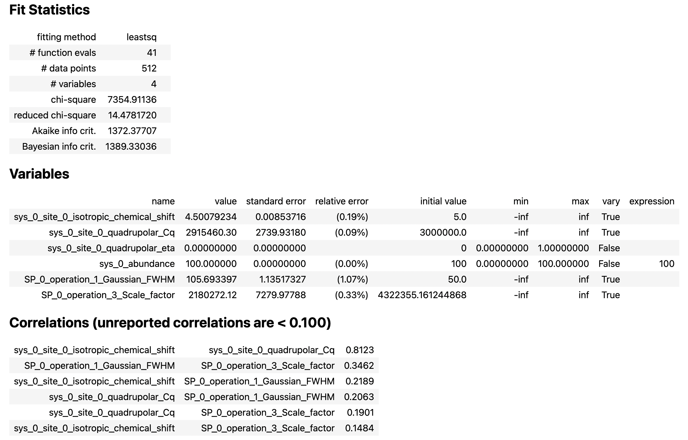
From the printout of the MinimizerResult above, you can find the best-fit parameters and their associated uncertainties from least-squares analysis.

Warning

A word of caution about best-fit parameter uncertainties: If the model is accurate, then you expect the residuals to be pure noise, i.e., a histogram of the residuals should arise from a Gaussian parent distribution with a mean of zero. Therefore, at the very least, you should inspect a plot of the residuals and, even better, check that a histogram of the residuals is consistent with a Gaussian parent distribution.

If this is not true, then the parameter uncertainties from the least-squares analysis will be underestimated. Such discrepancies between the experimental and simulated spectra can often arise from measurement artifacts, e.g., receiver deadtimes, non-uniform excitation, etc. They can also arise from an inadequate model (spin systems and method) for the spectrum.

Compare experimental and best-fit spectra with residuals¶

You can now plot the experimental and best-fit simulated spectra along with the residuals. Use the MRSimulator utility function bestfit() and residuals() to extract the best-fit simulation and the residuals as CSDM instances.

best_fit = sf.bestfit(sim, processor)[0].real
residuals = sf.residuals(sim, processor)[0].real

# Plot the spectrum
plt.figure(figsize=(6, 3.0))
ax = plt.subplot(projection="csdm")
ax.plot(exp_spectrum, label="Experiment")
ax.plot(best_fit, alpha=0.75, label="Best Fit")
ax.plot(residuals, alpha=0.75, label="Residuals")
ax.set_xlim(-20, 10)
plt.legend()
plt.grid()
plt.tight_layout()
plt.show()

(png, hires.png, pdf)

The Minimizer will improve the fit parameters even if the initial parameters are far from the best-fit values. However, if the initial parameters are too far away, the Minimizer may not reach the best-fit parameters in a single run. If you think that may be the case, you can re-extract a new initial guess from the Simulator and SignalProcessor instances using make_LMFIT_params(), create and initialize a new Minimizer instance as before, and run again, i.e., rerun the code starting at the beginning of this section. You may see that the fit improves and gives a lower chi-squared value.

In the least-square analysis above, you had locked the quadrupolar asymmetry parameter to a value of zero, which is reasonably close to the true value. At such low values, the quadrupolar asymmetry parameter is correlated to the Gaussian line broadening FWHM in the fit. Set the quadrupolar asymmetry parameter to be a fit parameter, and rerun the analysis.

fit_parameters["sys_0_site_0_quadrupolar_eta"].value = 0.05
fit_parameters["sys_0_site_0_quadrupolar_eta"].vary = True

minner = Minimizer(
    sf.LMFIT_min_function,
    fit_parameters,
    fcn_args=(sim, processor, sigma),
    fcn_kws={"opt": opt}
)
result = minner.minimize(method="powell")
result = minner.minimize(
    params=result.params, method="leastsq"
)

best_fit = sf.bestfit(sim, processor)[0].real
residuals = sf.residuals(sim, processor)[0].real

# Plot the spectrum
plt.figure(figsize=(6, 3.0))
ax = plt.subplot(projection="csdm")
ax.plot(exp_spectrum, label="Experiment")
ax.plot(best_fit, alpha=0.75, label="Best Fit")
ax.plot(residuals, alpha=0.75, label="Residuals")
ax.set_xlim(-20, 10)
plt.legend()
plt.grid()
plt.tight_layout()
plt.show()

(png, hires.png, pdf)

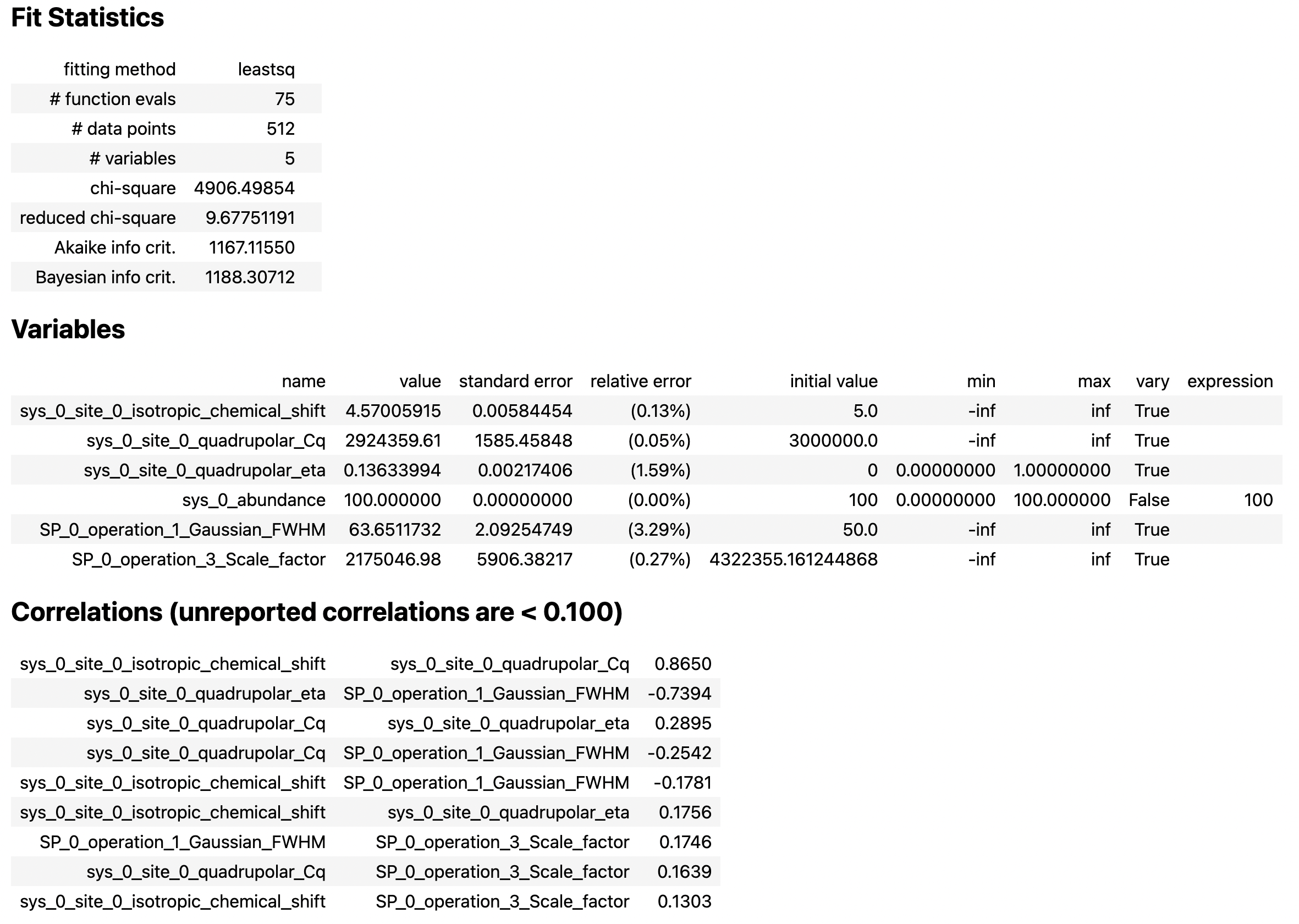
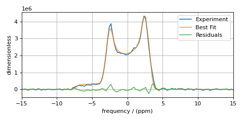
You see a slight improvement in the fit, with the asymmetry parameter increasing from 0 to 0.136, and the Gaussian FWHM decreased from 106 to 63 Hz. The MinimizerResult printout also shows a correlation of -0.74 between these two parameters.

We close this section by noting that a compelling feature of mrsimulator and LMFit is that you can perform a simultaneous spectra fit from different methods for a single set of spin system parameters. Check out all the examples in the Fitting (Least Squares) Gallery, notably the ¹³C MAS NMR of Glycine (CSA) multi-spectra fit example for fitting one set of spin systems to multiple spectra.