Spin System¶

Overview¶

At the heart of any mrsimulator calculation is the definition of a SpinSystem object describing the sites and couplings within a spin system. Each Simulator object holds a list of SpinSystem objects which are used to calculate frequency contributions.

mrsimulator faces the same limitation faced by all other NMR simulation codes: the computational cost increases exponentially with the number of couplings between sites in a spin system. In liquids, where isotropic molecular motion averages away intermolecular anisotropic couplings, the situation is more tractable as only the intramolecular isotropic J couplings remain.

In solids, where no such isotropic motion exists, the situation is more problematic. In solids that are dilute in NMR-active nuclei is often possible to build a set of SpinSystem objects that can accurately model a spectrum. In solids that are not dilute in NMR-active nuclei, there are still situations where one can build approximately accurate spin systems models. One such case is when the individual anisotropic spin interactions, such as the shielding (shift) anisotropy or the quadrupolar couplings, dominant the spectrum, i.e., they are significantly larger than any dipolar couplings. This can happen for spin 1/2 nuclei in static samples or samples spinning away from the magic-angle. In the case of half-integer quadrupolar nuclei, this can also happen for a central transition spectrum that is significantly broadened by second-order quadrupolar effects. Another case is when an experimental method can successfully decouple the effects of dipolar couplings from the spectrum, rendering it similar to that of a dilute spin system. This can be achieved through rapid sample rotation, a pulse sequence, or some clever combination of the two. In all such cases, any effects of residual dipolar couplings on the spectrum are usually modeled as an ad-hoc Gaussian lineshape convolution.

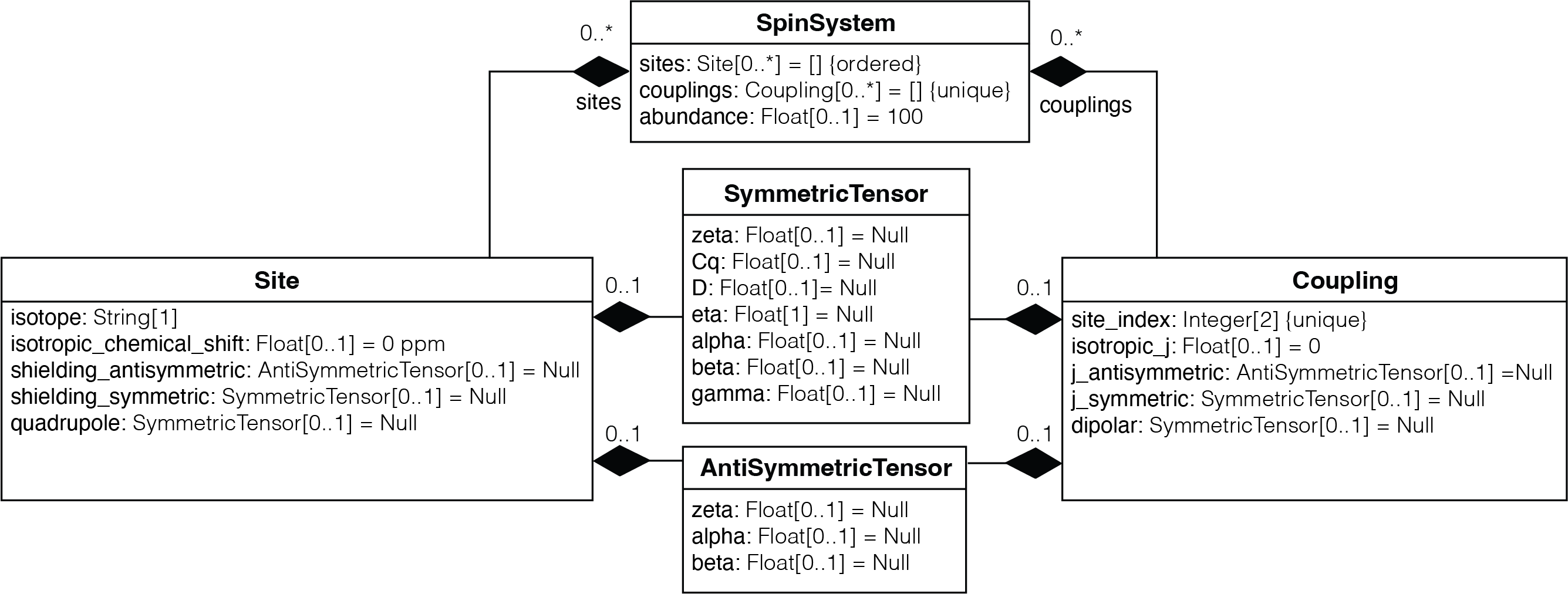
A SpinSystem object is organized according to the UML diagram below.

Note

In UML (Unified Modeling Language) diagrams, each class is represented with a box that contains two compartments. The top compartment contains the name of the class, and the bottom compartment contains the attributes of the class. Default attribute values are shown as assignments. A composition is depicted as a binary association decorated with a filled black diamond. Inheritance is shown as a line with a hollow triangle as an arrowhead.

Site¶

A site object holds single-site NMR interaction parameters, which include the nuclear shielding and quadrupolar interaction parameters. Consider the example below of a Site object for a deuterium nucleus created in Python.

# Import objects for the Site
from mrsimulator import Site
from mrsimulator.spin_system.tensors import SymmetricTensor

# Create the site object
H2_site = Site(
    isotope="2H",
    isotropic_chemical_shift=4.1,  # in ppm
    shielding_symmetric=SymmetricTensor(
        zeta=12.12,  # in ppm
        eta=0.82,
        alpha=5.45,  # in radians
        beta=4.82,  # in radians
        gamma=0.5,  # in radians
    ),
    quadrupolar=SymmetricTensor(
        Cq=1.47e6,  # in Hz
        eta=0.27,
        alpha=0.212,  # in radians
        beta=1.231,  # in radians
        gamma=3.1415,  # in radians
    ),
)

The isotope key holds the spin isotope, here given a value of "2H". The isotropic_chemical_shift is the isotropic chemical shift of the site isotope, \(^2\text{H}\), here given as 4.1 ppm. We have additionally defined an optional shielding_symmetric key, whose value is a second-rank traceless symmetric nuclear shielding tensor represented by a SymmetricTensor object.

Note

We parameterize a SymmetricTensor using the Haeberlen convention with parameters zeta and eta, defined as the shielding anisotropy and asymmetry, respectively. The Euler angle orientations, alpha, beta, and gamma are the relative orientation of the nuclear shielding tensor from a common reference frame.

Since deuterium is a quadrupolar nucleus, \(I>1/2\), there also can be a quadrupolar coupling interaction between the nuclear quadrupole moment and the surrounding electric field gradient (EFG) tensor, defined in the optional quadrupolar key. An EFG tensor is a second-rank traceless symmetric tensor, and we describe its coupling to a quadrupolar nucleus with Cq and eta, i.e., the quadrupolar coupling constant and asymmetry parameter, respectively. Additionally, we use the Euler angle orientations, alpha, beta, and gamma, which are the relative orientation of the EFG tensor from a common reference frame.

See Table 2 and Table 4 for further information on the Site and SymmetricTensor objects and their attributes, respectively.

Also, all objects in mrsimulator have the attribute property_units which provides the units for all class properties.

print(Site().property_units)
# {'isotropic_chemical_shift': 'ppm'}

print(SymmetricTensor().property_units)
# {'zeta': 'ppm', 'Cq': 'Hz', 'D': 'Hz', 'alpha': 'rad', 'beta': 'rad', 'gamma': 'rad'}

Coupling¶

A coupling object holds two site NMR interaction parameters, which can include the J-coupling and the dipolar coupling interaction parameters. Consider the example below of a Coupling object between two sites

# Import the Coupling object
from mrsimulator import Coupling

coupling = Coupling(
    site_index=[0, 1],
    isotropic_j=15,  # in Hz
    j_symmetric=SymmetricTensor(
        zeta=12.12,  # in Hz
        eta=0.82,
        alpha=2.45,  # in radians
        beta=1.75,  # in radians
        gamma=0.15,  # in radians
    ),
    dipolar=SymmetricTensor(
        D=1.7e3,  # in Hz
        alpha=0.12,  # in radians
        beta=0.231,  # in radians
        gamma=1.1415,  # in radians
    ),
)

The site_index key holds a list of two integers corresponding to the index of the two coupled sites in the ordered list sites within the SpinSystem object. The ordering of the integers in site_index is irrelevant.

The value of the isotropic_j is the isotropic J-coupling, here given as 15 Hz. We have additionally defined an optional j_symmetric key, whose value holds a SymmetricTensor object representing the traceless 2nd-rank symmetric J-coupling tensor.

Additionally, the dipolar coupling interaction between the coupled nuclei is defined with an optional dipolar key. A dipolar tensor is a second-rank traceless symmetric tensor, and we describe the dipolar coupling constant with the parameter D. The Euler angle orientations, alpha, beta, and gamma are the relative orientation of the dipolar tensor from a common reference frame.

Note

All frequency contributions from spin-spin couplings are calculated in the weak-coupling limit.

See Table 3 and Table 4 for further information on the Site and SymmetricTensor objects and their attributes, respectively.

SpinSystem¶

The SpinSystem object is a collection of sites and couplings. Below are examples of different spin systems along with discussion on each attribute.

Single Site Spin System¶

Here we create a relatively unexciting single site proton spin system

# Import the SpinSystem object
from mrsimulator import SpinSystem

H1_site = Site(isotope="1H")

single_site_sys = SpinSystem(
    name="1H spin system",
    description="A single site proton spin system",
    sites=[H1_site],
    abundance=80,  # percentage
)

We find four keywords at the root level of our SpinSystem object definition: name, description, sites, and abundance. The value of the name key is the optional name of the spin system. Likewise, the value of the description key is an optional string describing the spin system.

The value of the sites key is a list of Site objects. Here, this list is simply the single object, H1_site. The value of the abundance key is the abundance of the spin system, here given a value of 80%. If the abundance key is omitted, the abundance defaults to 100%.

See Table 1 for further description of the SpinSystem class and its attributes.

Multi Site Spin System¶

To create a spin system with more than one site, we simply add more site objects to the sites list. Here we create a \(^{13}\text{C}\) site and add it along with the previous proton site to a new spin system.

# Create the new Site object
C13_site = Site(
    isotope="13C",
    isotropic_chemical_shift=-53.2,  # in ppm
    shielding_symmetric=SymmetricTensor(
        zeta=90.5,  # in ppm
        eta=0.64,
    ),
)

# Create a new SpinSystem object with both Sites
multi_site_sys = SpinSystem(
    name="Multi site spin system",
    description="A spin system with multiple sites",
    sites=[H1_site, C13_site],
    abundance=0.148,  # percentage
)

Again we see the optional name and description attributes. The sites attribute is now a list of two Site objects, the previous \(^1\text{H}\) site and the new \(^{13}\text{C}\) site. We have also set the abundance of this spin system to 0.148%. By leveraging the abundance attribute, multiple spin systems with varying abundances can be simulated together. See our Isotopomers Example where isotopomers of varying abundance are simulated in tandem.

Coupled Spin System¶

To create couplings between sites, we simply need to add a list of Coupling objects to a spin system. Below we create a \(^{2}\text{H}\) and \(^{13}\text{C}\) site as well as a coupling between them.

# Create site objects
H2_site = Site(
    isotope="2H",
    isotropic_chemical_shift=4.1,  # in ppm
    shielding_symmetric=SymmetricTensor(
        zeta=12.12,  # in ppm
        eta=0.82,
        alpha=5.45,  # in radians
        beta=4.82,  # in radians
        gamma=0.5,  # in radians
    ),
    quadrupolar=SymmetricTensor(
        Cq=1.47e6,  # in Hz
        eta=0.27,
        alpha=0.212,  # in radians
        beta=1.231,  # in radians
        gamma=3.1415,  # in radians
    ),
)
C13_site = Site(
    isotope="13C",
    isotropic_chemical_shift=-53.2,  # in ppm
    shielding_symmetric=SymmetricTensor(
        zeta=90.5,  # in ppm
        eta=0.64,
    ),
)

# Create coupling object
H2_C13_coupling = Coupling(
    site_index=[0, 1],
    isotropic_j=15,  # in Hz
    j_symmetric=SymmetricTensor(
        zeta=12.12,  # in Hz
        eta=0.82,
        alpha=2.45,  # in radians
        beta=1.75,  # in radians
        gamma=0.15,  # in radians
    ),
    dipolar=SymmetricTensor(
        D=1.7e3,  # in Hz
        alpha=0.12,  # in radians
        beta=0.231,  # in radians
        gamma=1.1415,  # in radians
    ),
)

We now have the site objects and the coupling object to make a coupled spin system. We now construct such a spin system.

coupled_spin_system = SpinSystem(sites=[H2_site, C13_site], couplings=[H2_C13_coupling])

In contrast to the previous examples, we have omitted the optional name, description, and abundance keywords. The name and description for coupled_spin_system will both be None and the abundance will be 100%.

A list of Coupling objects passed to the couplings keywords. The site_index attribute of H2_C13_coupling correspond to the index of H2_site and C13_site in the sites list. If we were to add more sites, site_index might need to be updated to reflect the index H2_site` and C13_site in the sites list. Again, our Isotopomers Example has good usage cases for multiple couplings in a spin system.

Attribute Summaries¶

Table 1 The attributes of a SpinSystem object.¶
Attributes	Type	Description
`name`	String	An optional attribute with a name for the spin system. Naming is a good practice as it improves the readability, especially when multiple spin systems are present. The default value is an empty string.
`label`	String	An optional attribute giving a label to the spin system. Like `name`, it has no effect on a simulation and is purely for readability.
`description`	String	An optional attribute describing the spin system. The default value is an empty string.
`sites`	List	An optional list of Site objects. The default value is an empty list.
`couplings`	List	An optional list of coupling objects. The default value is an empty list.
`abundance`	String	An optional quantity representing the abundance of the spin system. The abundance is given as percentage, for example, `25.4` for 25.4%. This value is useful when multiple spin systems are present. The default value is `100`.

Table 2 The attributes of a Site object.¶
Attribute name	Type	Description
`name`, `label`, and `description`	String	All three are optional attributes giving context to a Site object. The default value for all three is an empty string.
`isotope`	String	A required isotope string given as the atomic number followed by the isotope symbol, for example, `13C`, `29Si`, `27Al`, and so on.
`isotropic_chemical_shift`	ScalarQuantity	An optional physical quantity describing the isotropic chemical shift of the site. The value is given in ppm, for example, `10` for 10 ppm. The default value is `0`.
`shielding_symmetric`	SymmetricTensor	An optional object describing the second-rank traceless symmetric nuclear shielding tensor following the Haeberlen convention. The default is `None`. See the description for the SymmetricTensor object.
`quadrupolar`	SymmetricTensor	An optional object describing the second-rank traceless electric quadrupole tensor. The default is `None`. See the description for the SymmetricTensor object.

Table 3 The attributes of a Coupling object.¶
Attribute name	Type	Description
`site_index`	List of two integers	A required list with integers corresponding to the site index of the coupled sites, for example, [0, 1], [2, 1]. The order of the integers is irrelevant.
`isotropic_j`	ScalarQuantity	An optional physical quantity describing the isotropic J-coupling in Hz. The default value is `0`.
`j_symmetric`	SymmetricTensor	An optional object describing the second-rank traceless symmetric J-coupling tensor following the Haeberlen convention. The default is `None`. See the description for the SymmetricTensor object.
`dipolar`	SymmetricTensor	An optional object describing the second-rank traceless dipolar tensor. The default is `None`. See the description for the SymmetricTensor object.

Table 4 The attributes of a SymmetricTensor object.¶
Attribute name	Type	Description
`zeta` or `Cq` or `D`	ScalarQuantity	A required quantity. Nuclear shielding: The shielding anisotropy, `zeta`, calculated using the Haeberlen convention. The value is a physical quantity given in ppm, for example, `10` Electric quadrupole: The quadrupole coupling constant, `Cq`. The value is a physical quantity given in units of Hz, for example, `3.1e6` for 3.1 MHz. J-coupling: The J-coupling anisotropy, `zeta`, calculated using the Haeberlen convention. The value is a physical quantity given in Hz, for example, `10` for 10 Hz. Dipolar-coupling: The dipolar-coupling constant, `D`. The value is a physical quantity given in Hz, for example, `9e6` for 9 kHz.
`eta`	Float	A required asymmetry parameter calculated using the Haeberlen convention, for example, `0.75`. The parameter is set to zero for the dipolar tensor.
`alpha`	ScalarQuantity	An optional Euler angle, \(\alpha\). For example, `2.1` for 2.1 radians. The default value is `0`.
`beta`	ScalarQuantity	An optional Euler angle, \(\beta\). For example, `1.5708` for 90 degrees. The default value is `0`.
`gamma`	ScalarQuantity	An optional Euler angle, \(\gamma\). For example, `0.5` for 0.5 radians. The default value is `0`.