Method
While MRSimulator’s organization of the SpinSystem class and its composite classes, Site and Coupling, are easily understood by anyone familiar with the underlying physical concepts, the organization of the Method class in MRSimulator and its related composite classes require a more detailed explanation of their design. This section assumes that you are already familiar with the topics covered in the Introduction sections Getting Started, Isotopomers Example, and Least-Squares Fitting Example.
Note
Before writing a custom Method, check if any of our pre-built methods in the Methods Library can serve your needs.
Overview
An experimental NMR method involves a sequence of RF pulses, free evolution periods, and sample motion. The Method class in MRSimulator models the spectrum from an NMR pulse sequence. The Method class is designed to be versatile in its ability to model spectra from various multi-pulse NMR methods using concepts from the symmetry pathway approach where a pulse sequence is understood in terms of a set of desired (and undesired) transition pathways. Each transition pathway is associated with a single resonance in a multi-dimensional NMR spectrum. The transition pathway signal encodes information about the spin system interactions in its amplitude and correlated frequencies. Consider the illustration of a 2D pulse sequence shown below, where a desired signal for the method is associated with a particular transition pathway, \({\hat{A} \rightarrow \hat{B} \rightarrow \hat{C} \rightarrow \hat{D} \rightarrow \hat {E} \rightarrow \hat{F}}\).
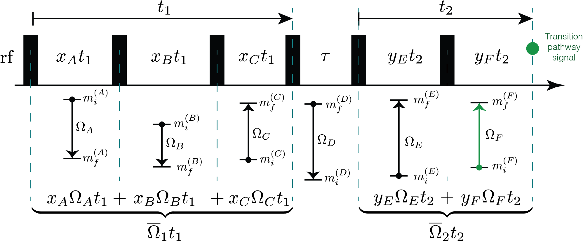
Figure 24 An illustration of a two-dimensional NMR pulse sequence leading up to the acquisition of the signal from a transition pathway
Here, the first spectral dimension, i.e., the Fourier transform of the transition pathway signal as a function of \(t_1\), derives its average frequency, \(\overline{\Omega}_1\), from a weighted average of the \(\hat{A}\), \(\hat{B}\), and \(\hat{C}\) transition frequencies. The second spectral dimension, i.e., the FT with respect to \(t_2\), derives its average frequency, \(\overline{\Omega}_2\), from a weighted average of the \(\hat{E}\), and \(\hat{F}\) transition frequencies. Much of the experimental design and implementation of an NMR method is in identifying the desired transition pathways and finding ways to acquire their signals while eliminating all undesired transition pathway signals.
While NMR measurements occur in the time domain, MRSimulator simulates the corresponding multi-dimensional spectra directly in the frequency domain. The Method class in MRSimulator needs only a few details of the NMR pulse sequence to generate the spectrum. It mimics the result of the pulse sequence given the desired transition pathways and their complex amplitudes and average frequencies in each spectroscopic dimension of the dataset. To this end, the Method class is organized according to the UML diagram below.
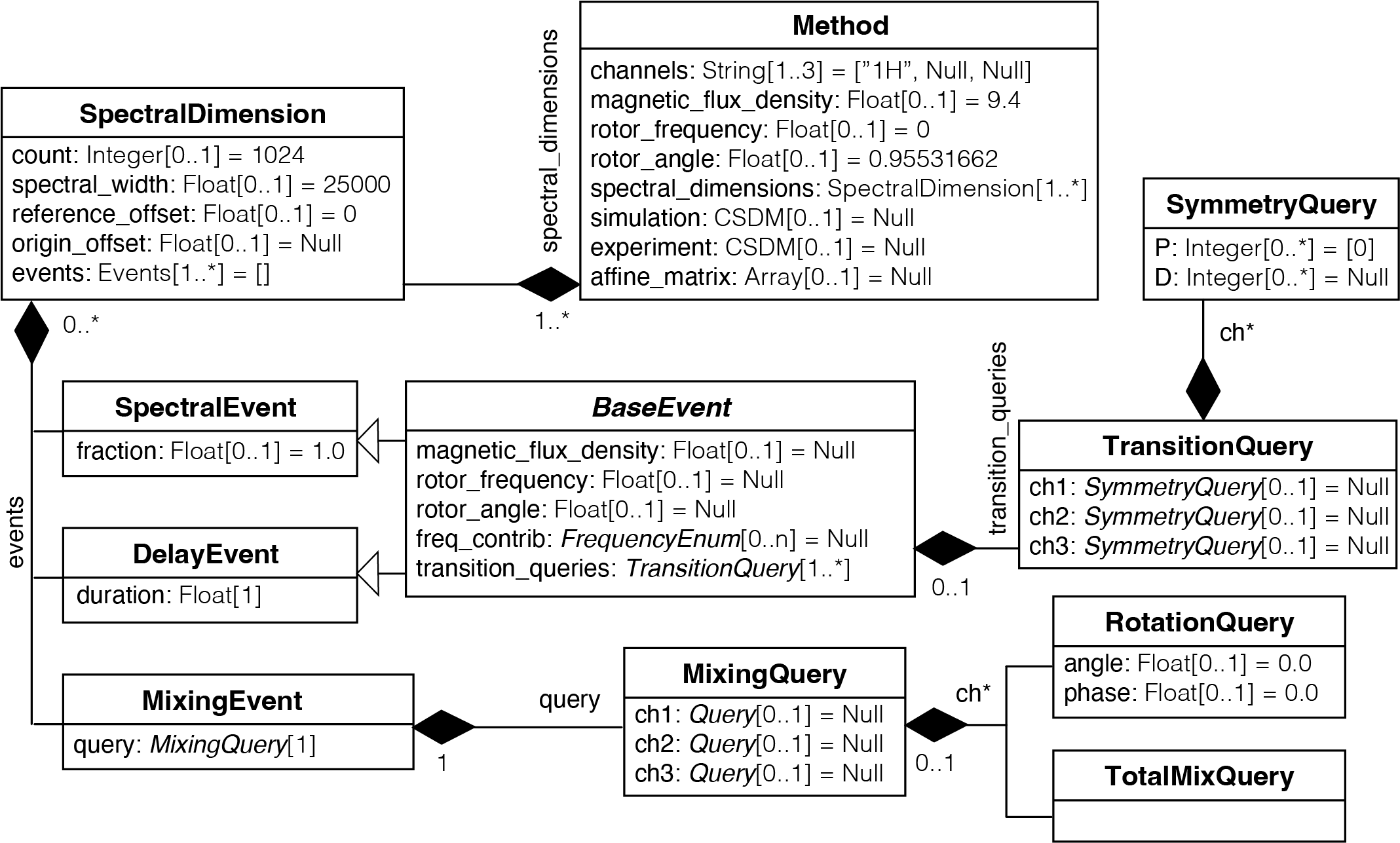
Figure 25 Unified Modeling Language class diagram of the Method Class in MRSimulator.
Note
In UML (Unified Modeling Language) diagrams, each class is represented with a box that contains two compartments. The top compartment has the class’s name, and the bottom compartment contains the class’s attributes. Default attribute values are shown as assignments. A composition is depicted as a binary association decorated with a filled black diamond. Inheritance is shown as a line with a hollow triangle as an arrowhead.
At the heart of a Method class, assigned to its attribute
spectral_dimensions, is an ordered list of SpectralDimension instances
in the same order as the time evolution dimensions of the experimental NMR
sequence. In each SpectralDimension instance is an ordered list of Events
instance assigned to the attribute events; Event classes are divided
into three types: (1) SpectralEvent(), (2)
DelayEvent(), and (3)
RotationEvent(). This ordered list of Event instances
is used to select the desired transition pathways and determine their average
frequency and complex amplitude in the SpectralDimension.
SpectralEvent and DelayEvent classes define which transitions are
observed during the event and under which transition-dependent frequency
contributions they evolve. No coherence transfer among transitions or
populations occurs in a spectral or delay event. The transition-dependent
frequency contributions during an Event are selected from a list of
enumeration literals and placed in the freq_contrib
attribute of the event. Frequency contributions can be individually excluded by
placing an exclamation mark in front of the string representing the enumeration
literal. If freq_contrib is left unspecified, i.e., the
value of freq_contrib is set to None, a default list holding the
enumeration literals for all contributions is generated for the event.
Note
All frequency contributions from direct and indirect spin-spin couplings are calculated in the weak-coupling limit in MRSimulator.
Additionally, the user can affect transition frequencies during a spectral or
delay event by changing other measurement attributes: rotor_frequency,
rotor_angle, and magnetic_flux_density. If left unspecified, these
attributes default to the values of the identically named global attributes in
the Method instance. SpectralEvent instances use the fraction attribute to
calculate the weighted average frequency during the spectral dimension for each
selected transition pathway.
Inside SpectralEvent and DelayEvent instances, is a list of
TransitionQuery() instances (vide infra)
which determine which transitions are observed during the event. Method
instances in MRSimulator are general-purpose because they are designed for an
arbitrary spin system, i.e., a method does not know the spin system in advance.
When designing a Method instance, you cannot identify and select a transition
through its initial and final eigenstate quantum numbers. Transition selection
is done through TransitionQuery and
SymmetryQuery() instances during individual
spectral or delay events. TransitionQuery instances can hold a
SymmetryQuery instance in the attributes ch1, ch2, or ch3, which act on
specific isotopes defined by the channels attribute in Method. It is
only during a simulation that the Method instance uses its TransitionQuery
instances to determine the selected transition pathways for a given SpinSystem
instance by the initial and final eigenstate quantum numbers of each transition.
Between adjacent FreeEvent instances, MRSimulator defaults
to total mixing, i.e., connecting all selected transitions in the two adjacent
spectral or delay events. This default behavior can be overridden by placing an
explicit RotationEvent() instance between such events.
The RotationEvent instance holds Rotation()
instances in the attributes ch1, ch2, or ch3, which act on specific
isotopes defined by the channels attribute in Method. The Rotation class
determines the coherence transfer amplitude between transitions.
In this guide to designing custom Method instances, we begin with a brief review of the relevant Symmetry Pathway concepts employed in MRSimulator. This review is necessary for understanding (1) how transitions are selected during spectral and delay events and (2) how average signal frequencies and amplitudes in each spectral dimension are determined. We outline the procedures for designing and creating TransitionQuery and RotationEvent instances for single- and multi-spin transitions and how to use them to select the transition pathways with the desired frequency and amplitudes in each spectral dimension of your custom Method instance. In multi-dimensional spectra, we illustrate how the desired frequency correlation can sometimes be achieved by using an appropriate affine transformation. We also examine how changing the frequency contributions in SpectralEvent of DelayEvent instances can be used to obtain the desired frequency and amplitude behavior. The ability to select frequency contributions can often reduce the number of events needed in the design of your custom Method instance.
Theoretical Background
Before giving details on how to create a custom Method instance, we review a few key concepts about spin transitions and transition symmetry functions.
The number of quantized energy eigenstates for \(N\) coupled nuclei is
where \(I_u\) is the total spin angular momentum quantum number of the \(u\text{th}\) nucleus. The transition from quantized energy level \(E_i\) to \(E_j\) is one of
possible transitions between the \(\Upsilon\) levels. Here we count \(i \rightarrow j\) and \(j \rightarrow i\) as different transitions. For example, a single spin with angular momentum quantum number \(I=3/2\) will have \(\Upsilon_{\left\{ 3/2 \right\}} = 2I+1 = 4\) energy levels and \(\mathcal{N}_{\left\{ 3/2 \right\}} = 2I(2I+1) = 12\) possible NMR transitions. A two spin system, with quantum numbers \(I = 1/2\) and \(S = 1/2\), will have
energy levels and
possible NMR transitions. We write a transition (coherence) from state \(i\) to \(j\) using the outer product notation \(\ketbra{j}{i}\). In MRSimulator, all simulations are performed in the high-field limit and further, assume that all spin-spin couplings are in the weak limit.
To write a custom Method in MRSimulator, you’ll need to determine the desired transition pathways and select the desired transitions during each SpectralEvent or DelayEvent. Keep in mind, however, that the Method class is designed without any details of the spin systems upon which it will act. For example, in the density matrix of a spin system ensemble, one could easily identify a transition by its row and column indexes. However, those indexes depend on the spin system and how the spins and their eigenstates have been assigned to those indexes. Instead, we need a spin-system agnostic approach for selecting transitions.
Spin Transition Symmetry Functions
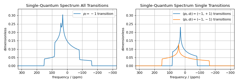
One way you can select a subset of single-spin transitions if you don’t know the energy eigenstate quantum numbers is to request all transitions whose single-spin transition symmetry function, \(\text{p}_I\) is \(-1\), i.e.,
The \(\text{p}_I\) single-spin transition symmetry function is also known as the single-spin coherence order of the transition.
Note
In the high field limit, only single-spin transitions with \({\text{p}_I = \pm 1}\) are directly observed. Since the evolution frequencies of the \(\ketbra{j}{i}\) and \(\ketbra{i}{j}\) transitions are equal in magnitude but opposite in sign, the convention is to only present the \({\text{p}_I = - 1}\) transition resonances in single-quantum spectra.
By selecting only single-spin transitions with \(\text{p}_I = -1\), you get all the “observed” transitions from the set of all possible transitions. Similarly, you can use \(\text{p}_I\) to select any subset of single-spin transitions, such as double-quantum \((\text{p}_I = \pm 2)\) transitions, triple-quantum \((\text{p}_I = \pm 3)\) transitions, etc.
While specifying \(\text{p}_I\) alone is not enough to select an individual single-spin transition, any individual single-spin transition can be identified by a combination of \(\text{p}_I\) and the single-spin transition symmetry function \(\text{d}_I\), given by
You can verify this from the values of \(\text {p}_I\) and \(\text{d}_I\) for all single-spin transitions for \(I=1\), \(I=3/2\) and \(I=5/2\) shown below. Note that \(\text{d}_I = 0\) for all transitions in a \(I=1/2\) nucleus.
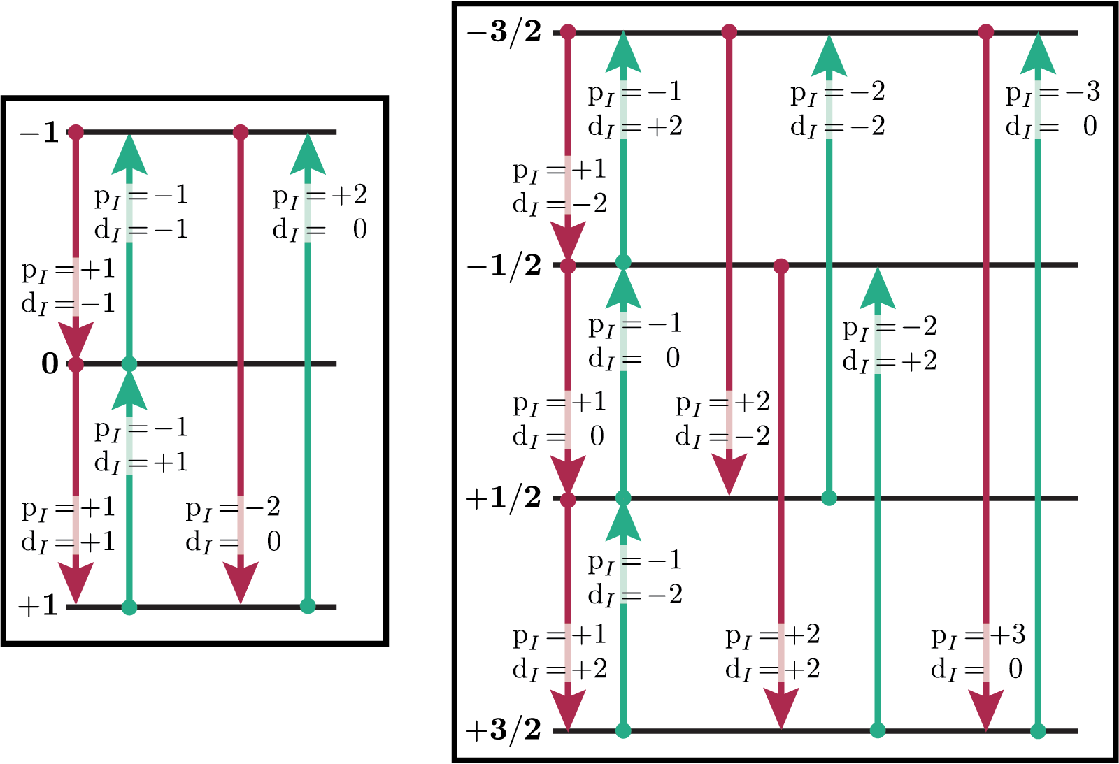
Figure 26 Energy level diagrams of a spin \(I=1\) nucleus (left) and spin \(I=3/2\) nucleus (right). Arrows beginning at the initial state and ending at the final state represent transitions. Transitions are labeled with their corresponding \(\text{p}_I\) and \(\text{d}_I\) transition symmetry function values.
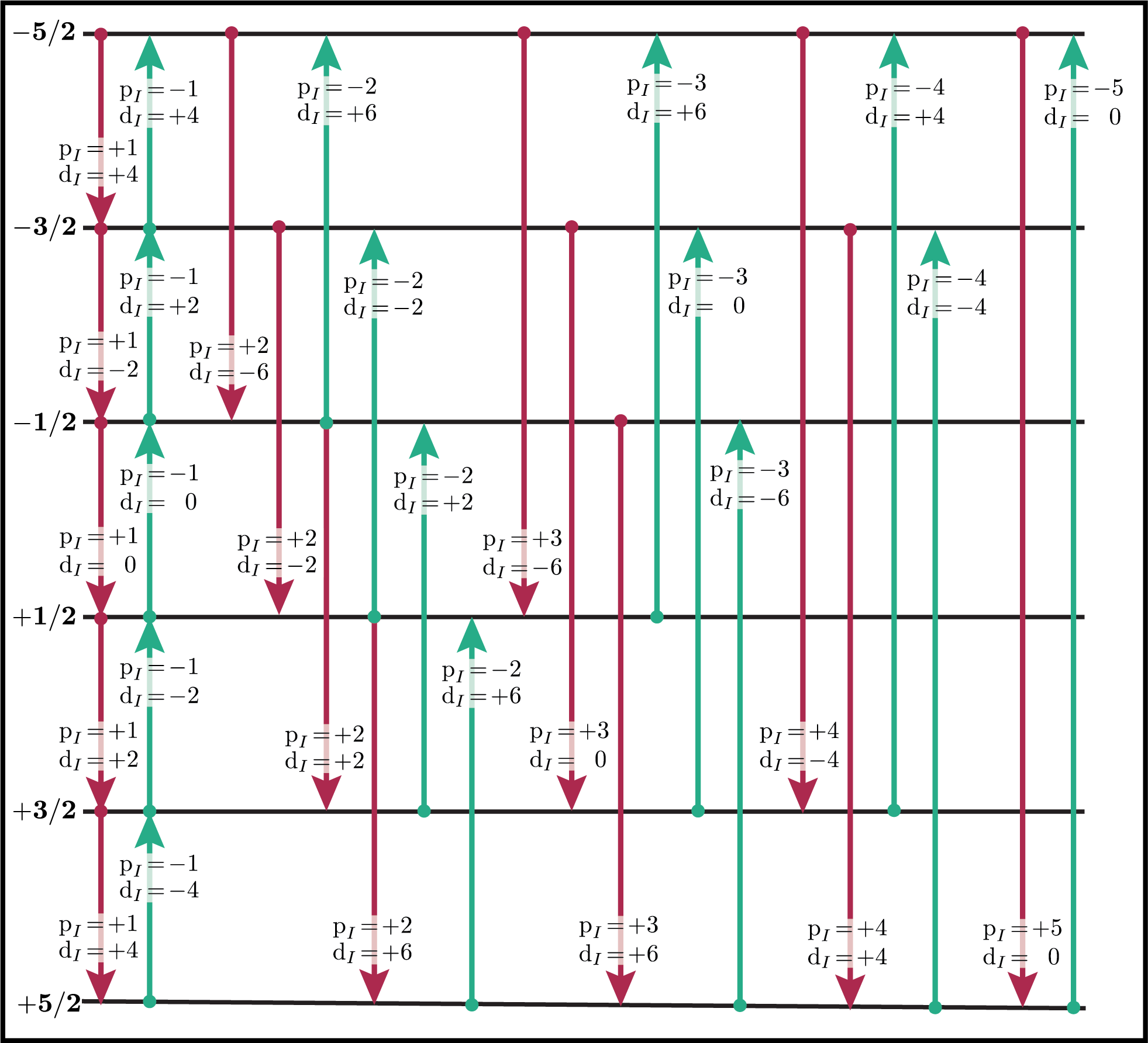
Figure 27 Energy level diagram of a spin \(I=5/2\) nucleus. Arrows beginning at the initial state and ending at the final state represent transitions. Transitions are labeled with their corresponding \(\text{p}_I\) and \(\text{d}_I\) spin transition symmetry function values.
For a summary of spin transition symmetry functions in NMR, click on the disclosure button below.
Spin Transition Symmetry Functions
Note
In the symmetry pathway approach, the idea of coherence order is extended to form a complete set of spin transition symmetry functions, \(\xi_\ell (i,j)\), given by
where the \(\hat{T}_{\ell,0}\) are irreducible tensor operators. The function symbol \(\xi_\ell(i,j)\) is replaced with the lower-case symbols \(\mathbb{p}(i,j)\), \(\mathbb{d}(i,j)\), \(\mathbb{f} (i,j)\), \(\ldots\), i.e., we follow the spectroscopic sub-shell letter designations:
To simplify usage in figures and discussions, we scale the transition symmetry functions to integer values according to
The \(\ell=0\) function is dropped as it always evaluates to zero. For a single spin, \(I\), a complete set of functions is defined up to \(\ell = 2I\).
For weakly coupled nuclei, we define the transition symmetry functions
Replacing the symmetry function symbol using sub-shell letter designations becomes more cumbersome in this case. When the \(\ell\) values are zero on all nuclei except one, we identify these functions as
For weakly coupled homonuclear spins, it is also convenient to define
When the \(\ell\) values are zero on all nuclei except two, then we identify these functions by using a concatenation of sub-shell letter designations, e.g.,
Below is an energy level diagram of two coupled spin \(I=1/2\) nuclei with transition labeled according to their transition symmetry function values. Note that each transition has a unique set of transition symmetry function values.
Single-Spin Queries
Based on the review above, we now know for the spin \(I=1\), the transition \(\ketbra{-1}{0}\) can be selected with \({(\text{p}_I,\text{d}_I) = (-1,1)}\). In MRSimulator, this transition is selected during a SpectralEvent using the SymmetryQuery and TransitionQuery instances, as defined in the code below.
from mrsimulator.method.query import SymmetryQuery, TransitionQuery
from mrsimulator.method import SpectralEvent

symm_query = SymmetryQuery(P=[-1], D=[1])
trans_query = TransitionQuery(ch1=symm_query)
spec_event = SpectralEvent(transition_queries=[trans_query])
Note
Python dictionaries can also be used to instantiate MRSimulator classes. To do this, the dictionary must use the class’s attribute names as the key strings and be passed to a higher-level class. Since a SpectralEvent instance holds a list of TransitionQuery instances, the above code could have been written as
# Both SymmetryQuery and TransitionQuery instances as dict
symm_query_dict = {"P": [-1], "D": [1]}
trans_query_dict = {"ch1": symm_query_dict}

# Dictionary of TransitionQuery passed to SpectralEvent
spec_event = SpectralEvent(transition_queries=[trans_query_dict])
In the example above, the SymmetryQuery instance is created and assigned to
the TransitionQuery attribute ch1, i.e., it acts on the isotope in the
“first channel”. Recall that the channels attribute of the Method class
holds an ordered list of isotope strings. This list’s first, second, and third
isotopes are associated with ch1, ch2, and ch3, respectively.
Currently, MRSimulator only supports up to three channels, although this may
be increased in future versions.
The TransitionQuery instance goes into a list in the
transition_queries attribute of a SpectralEvent instance. The
SpectralEvent instance, in turn, is added to an ordered list in the events
attribute of a SpectralDimension instance. All this is illustrated in the code
below.
from mrsimulator import Site, Coupling, SpinSystem, Simulator
from mrsimulator import Method, SpectralDimension
from mrsimulator import signal_processor as sp
import matplotlib.pyplot as plt
import numpy as np

# Create a single Site and Spin System
deuterium = Site(
    isotope="2H",
    isotropic_chemical_shift=10,  # in ppm
    shielding_symmetric={"zeta": -80, "eta": 0.25},  # zeta in ppm
    quadrupolar={"Cq": 10e3, "eta": 0.0, "alpha": 0, "beta": np.pi / 2, "gamma": 0},
)
deuterium_system = SpinSystem(sites=[deuterium])

# This method selects all observable (p_I = –1) transitions
method_both_transitions = Method(
    channels=["2H"],
    magnetic_flux_density=9.4,  # in T
    spectral_dimensions=[
        SpectralDimension(
            count=512,
            spectral_width=40000,  # in Hz
            events=[SpectralEvent(transition_queries=[{"ch1": {"P": [-1]}}])],
        )
    ],
)

# This method selects observable (p_I = –1) transitions with d_I = 1
method_transition1 = Method(
    channels=["2H"],
    magnetic_flux_density=9.4,  # in T
    spectral_dimensions=[
        SpectralDimension(
            count=512,
            spectral_width=40000,  # in Hz
            events=[SpectralEvent(transition_queries=[{"ch1": {"P": [-1], "D": [1]}}])],
        )
    ],
)

# This method selects observable (p_I = –1) transitions with d_I = -1
method_transition2 = Method(
    channels=["2H"],
    magnetic_flux_density=9.4,  # in T
    spectral_dimensions=[
        SpectralDimension(
            count=512,
            spectral_width=40000,  # in Hz
            events=[SpectralEvent(transition_queries=[{"ch1": {"P": [-1], "D": [-1]}}])],
        )
    ],
)
# Simulate spectra for all three methods with spin system
sim = Simulator(
    spin_systems=[deuterium_system],
    methods=[method_both_transitions, method_transition1, method_transition2],
)
sim.run()

# Create SignalProcessor for Gaussian Convolution
processor = sp.SignalProcessor(
    operations=[sp.IFFT(), sp.apodization.Gaussian(FWHM="100 Hz"), sp.FFT()]
)
# Plot spectra from all three methods
fig, ax = plt.subplots(1, 2, figsize=(10, 3.5), subplot_kw={"projection": "csdm"}, sharey=True)
ax[0].plot(
    processor.apply_operations(dataset=sim.methods[0].simulation).real,
    label="$p_I = -1$ transition",
)
ax[0].set_title("Single-Quantum Spectrum All Transitions")
ax[0].legend()
ax[0].grid()
ax[0].invert_xaxis()  # reverse x-axis
ax[1].plot(
    processor.apply_operations(dataset=sim.methods[1].simulation).real,
    label="$(p_I,d_I) = (-1,+1)$ transitions",
)
ax[1].plot(
    processor.apply_operations(dataset=sim.methods[2].simulation).real,
    label="$(p_I,d_I) = (-1,-1)$ transitions",
)
ax[1].set_title("Single-Quantum Spectrum Single Transitions")
ax[1].legend()
ax[1].grid()
ax[1].invert_xaxis()  # reverse x-axis
plt.tight_layout()
plt.show()
Note
Whenever the D attribute is omitted, the SymmetryQuery allows
transitions with all values of \(\text{d}_I\). On the other hand, whenever
the P attribute is omitted, it defaults to P=[0], i.e., no selected
transitions on the assigned channel.
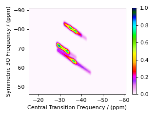
Selecting Symmetric Single-Spin Transitions
A notable case, particularly useful for half-integer quadrupolar nuclei, is that \(\text{d}_I = 0\) for all symmetric \((m \rightarrow - m)\) transitions, as these transitions are unaffected by the first-order quadrupolar coupling frequency contribution. The MQ-MAS experiment involves a 2D correlation of the two symmetric (\(\text{d}_I = 0\)) transitions, \(\ketbra{-\tfrac{1}{2}}{\tfrac{1}{2}}\), the so-called “central transition,” and \(\ketbra{-\tfrac{3}{2}}{\tfrac{3}{2}}\), the symmetric triple quantum transition. The code below is an example of a custom 2D method using two SpectralDimension instances, each holding a single SpectralEvent. The TransitionQuery instances select each transition in their respective SpectralDimension instances.
my_mqmas = Method(
    channels=["87Rb"],
    magnetic_flux_density=9.4,
    rotor_frequency=np.inf,  # in Hz (here, set to infinity)
    spectral_dimensions=[
        SpectralDimension(
            count=128,
            spectral_width=6e3,  # in Hz
            reference_offset=-9e3,  # in Hz
            label="Symmetric 3Q Frequency",
            events=[SpectralEvent(transition_queries=[{"ch1": {"P": [-3], "D": [0]}}])],
        ),
        SpectralDimension(
            count=256,
            spectral_width=6e3,  # in Hz
            reference_offset=-5e3,  # in Hz
            label="Central Transition Frequency",
            events=[SpectralEvent(transition_queries=[{"ch1": {"P": [-1], "D": [0]}}])],
        ),
    ],
)

# Create three sites in RbNO3
site1 = Site(
    isotope="87Rb",
    isotropic_chemical_shift=-27.4,  # ppm
    quadrupolar={"Cq": 1.68e6, "eta": 0.2},  # Cq in Hz
)
site2 = Site(
    isotope="87Rb",
    isotropic_chemical_shift=-28.5,  # ppm
    quadrupolar={"Cq": 1.94e6, "eta": 1},  # Cq in Hz
)
site3 = Site(
    isotope="87Rb",
    isotropic_chemical_shift=-31.3,  # ppm
    quadrupolar={"Cq": 1.72e6, "eta": 0.5},  # Cq in Hz
)

# No Couplings, so create a separate SpinSystem for each site.
sites = [site1, site2, site3]
RbNO3_spin_systems = [SpinSystem(sites=[s]) for s in sites]

sim = Simulator(spin_systems=RbNO3_spin_systems, methods=[my_mqmas])
sim.run()

# Apply Gaussian line broadening along both dimensions via convolution
gauss_convolve = sp.SignalProcessor(
    operations=[
        sp.IFFT(dim_index=(0, 1)),
        sp.apodization.Gaussian(FWHM="0.08 kHz", dim_index=0),
        sp.apodization.Gaussian(FWHM="0.22 kHz", dim_index=1),
        sp.FFT(dim_index=(0, 1)),
    ]
)
dataset = gauss_convolve.apply_operations(dataset=sim.methods[0].simulation)
In the code below, we use the imshow() from the
matplotlib.pyplot module to
return an image of the dataset on a 2D regular raster. We also use "gist_ncar_r" from
matpltolib’s included colormaps
to map the dataset amplitude to colors; the colorbar()
function provides the visualization of the dataset mapping to color to the right
of the plot.
plt.figure(figsize=(4, 3))
ax = plt.subplot(projection="csdm")
cb = ax.imshow(dataset.real / dataset.real.max(), aspect="auto", cmap="gist_ncar_r")
plt.colorbar(cb)
ax.invert_xaxis()
ax.invert_yaxis()
plt.tight_layout()
plt.show()
Warning
This custom method, as well as the built-in Multi-Quantum VAS methods, assumes uniform excitation and mixing of the multiple-quantum transition. In an experimental MQ-MAS measurement, excitation and mixing efficiencies depend on the ratio of the quadrupolar coupling constant to the RF field strength. Therefore, the relative integrated intensities of this simulation may not agree with the experiment.
Inspecting Transition and Symmetry Pathways
You can view the symmetry pathways that will be selected by your custom method
in a given spin system using the function
get_symmetry_pathways() as shown below.
from pprint import pprint
pprint(my_mqmas.get_symmetry_pathways("P"))
pprint(my_mqmas.get_symmetry_pathways("D"))
[SymmetryPathway(
    ch1(87Rb): [-3] ⟶ [-1]
    total: -3.0 ⟶ -1.0
)]
[SymmetryPathway(
    ch1(87Rb): [0] ⟶ [0]
    total: 0.0 ⟶ 0.0
)]
The method also has a related function plot() for generating a symmetry
pathway diagram of the method.
pathway_diagram = my_mqmas.plot()
pathway_diagram.show()

Similarly, you can view the transition pathway that will be selected by your custom method in a given
spin system using the function get_transition_pathways() as shown
below.
from pprint import pprint
pprint(my_mqmas.get_transition_pathways(SpinSystem(sites=[site1])))
[|-1.5⟩⟨1.5| ⟶ |-0.5⟩⟨0.5|, weight=(1+0j)]
Multi-Spin Queries
With more than one site in a spin system, things get a little more complicated with the SymmetryQuery class. Here, we review some important concepts associated with transition symmetry functions in coupled spin systems and see how the SymmetryQuery class is designed to work in such cases.
Single-Spin Single-Quantum Transitions
Consider the case of three weakly coupled proton sites. Here, the selection rule for observable transitions is
These correspond to the single-spin single-quantum transitions labeled \(\hat{A}_1\), \(\hat{A}_2\), \(\hat{A}_3\), \(\hat{A}_4\), \(\hat{M}_1\), \(\hat{M}_2\), \(\hat{M}_3\), \(\hat{M}_4\), \(\hat{X}_1\), \(\hat{X}_2\), \(\hat{X}_3\), and \(\hat{X}_4\) in the energy level diagram below.
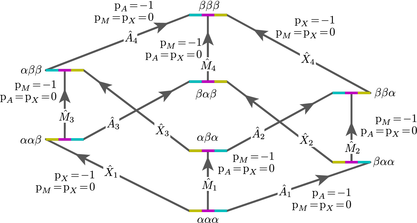
Figure 28 Energy level diagram for three coupled spin \(I=1/2\) nuclei. Arrows beginning at the initial state and ending at the final state represents the single-spin single-quantum transitions. Transitions are labeled with their corresponding single-spin \(\text{p}_i\) transition symmetry function values.
Keep in mind that the Method class does not know, in advance, the number of sites in a spin system.
The TransitionQuery for selecting these 12 single-spin single-quantum transitions is given in the code below.
# Create Site, Coupling and SpinSystem instances
site_A = Site(isotope="1H", isotropic_chemical_shift=0.5)
site_M = Site(isotope="1H", isotropic_chemical_shift=2.5)
site_X = Site(isotope="1H", isotropic_chemical_shift=4.5)
sites = [site_A, site_M, site_X]
coupling_AM = Coupling(site_index=[0, 1], isotropic_j=12)
coupling_AX = Coupling(site_index=[0, 2], isotropic_j=12)
coupling_MX = Coupling(site_index=[1, 2], isotropic_j=12)
couplings = [coupling_AM, coupling_AX, coupling_MX]
proton_system = SpinSystem(sites=sites, couplings=couplings)

# Custom Method instance emulating a one-pulse acquire experiment
method = Method(
    channels=["1H"],
    magnetic_flux_density=9.4,  # in T
    spectral_dimensions=[
        SpectralDimension(
            count=16000,
            spectral_width=1800,  # in Hz
            reference_offset=1000,  # in Hz
            label="$^{1}$H frequency",
            events=[SpectralEvent(transition_queries=[{"ch1": {"P": [-1]}}])],
        )
    ],
)

sim = Simulator(spin_systems=[proton_system], methods=[method])
sim.run()

# Add line broadening
processor = sp.SignalProcessor(
    operations=[sp.IFFT(), sp.apodization.Exponential(FWHM="1 Hz"), sp.FFT()]
)
plt.figure(figsize=(10, 3))  # set the figure size
ax = plt.subplot(projection="csdm")
ax.plot(processor.apply_operations(dataset=sim.methods[0].simulation).real)
ax.invert_xaxis()  # reverse x-axis
plt.tight_layout()
plt.grid()
plt.show()

The assignment of transitions in the spectrum above, from left to right, are \(\hat{X}_4, (\hat{X}_3, \hat{X}_2)\), and \(\hat{X}_1\) centered at 4.5 ppm, \(\hat{M}_4, (\hat{M}_3, \hat{M}_2)\), and \(\hat{M}_1\) centered at 2.5 ppm, and \(\hat{A}_4, (\hat{A}_3, \hat{A}_2)\), and \(\hat{A}_1\) centered at 0.5 ppm.
It is essential to realize that all sites having the same isotope appear
“indistinguishable” to a TransitionQuery instance. Recall that ch1 is
associated with the first isotope in the list of isotope strings assigned to the
Method attribute channels. When the TransitionQuery above is combined with
the SpinSystem instance with three \(^1\text{H}\) Sites, it must first expand
its SymmetryQuery into an intermediate set of spin-system-specific symmetry
queries, illustrated by each row in the table below.
Transitions |
\(\text{p}_A\) |
\(\text{p}_M\) |
\(\text{p}_X\) |
|---|---|---|---|
\(\hat{A}_1, \hat{A}_2, \hat{A}_3, \hat{A}_4\) |
–1 |
0 |
0 |
\(\hat{M}_1, \hat{M}_2, \hat{M}_3, \hat{M}_4\) |
0 |
–1 |
0 |
\(\hat{X}_1, \hat{X}_2, \hat{X}_3, \hat{X}_4\) |
0 |
0 |
–1 |
The intermediate spin-system-specific symmetry query in each row selects a subset of transitions from the complete set of transitions. The final set of selected transitions is obtained from the union of transition subsets from each spin-system-specific symmetry query.
The get_transition_pathways() function will allow
you to inspect the transitions selected by the Method
in terms of the initial and final Zeeman eigenstate quantum numbers.
from pprint import pprint
pprint(method.get_transition_pathways(proton_system))
[|-0.5, -0.5, -0.5⟩⟨-0.5, -0.5, 0.5|, weight=(1+0j),
|-0.5, -0.5, -0.5⟩⟨-0.5, 0.5, -0.5|, weight=(1+0j),
|-0.5, -0.5, 0.5⟩⟨-0.5, 0.5, 0.5|, weight=(1+0j),
|-0.5, 0.5, -0.5⟩⟨-0.5, 0.5, 0.5|, weight=(1+0j),
|-0.5, -0.5, -0.5⟩⟨0.5, -0.5, -0.5|, weight=(1+0j),
|-0.5, -0.5, 0.5⟩⟨0.5, -0.5, 0.5|, weight=(1+0j),
|0.5, -0.5, -0.5⟩⟨0.5, -0.5, 0.5|, weight=(1+0j),
|-0.5, 0.5, -0.5⟩⟨0.5, 0.5, -0.5|, weight=(1+0j),
|0.5, -0.5, -0.5⟩⟨0.5, 0.5, -0.5|, weight=(1+0j),
|-0.5, 0.5, 0.5⟩⟨0.5, 0.5, 0.5|, weight=(1+0j),
|0.5, -0.5, 0.5⟩⟨0.5, 0.5, 0.5|, weight=(1+0j),
|0.5, 0.5, -0.5⟩⟨0.5, 0.5, 0.5|, weight=(1+0j)]
To further illustrate how the TransitionQuery and SymmetryQuery instances work in a multi-site spin system, let’s examine a few more examples in the case of three weakly coupled proton sites.
Two-Spin Double-Quantum Transitions
In this spin system, there are six two-spin double-quantum transitions where \(\text{p}_{AMX} = \text{p}_{A} + \text{p}_{M} + \text{p}_{X} = -2\) and another six two-spin double-quantum transitions where \(\text{p}_{AMX} = \text{p}_{A} + \text{p}_{M} + \text{p}_{X} = +2\). The \(\text{p}_{AMX} = -2\) transitions are illustrated in the energy-level diagram below.
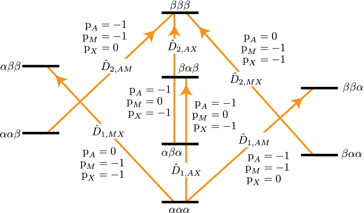
Figure 29 Energy level diagram for three coupled spin \(I=1/2\) nuclei. Arrows beginning at the initial state and end at the final state represent the two-spin double-quantum transitions. Transitions are labeled with their corresponding single-spin \(\text{p}_i\) transition symmetry function values.
The code below will select the six two-spin double-quantum transitions where \(\text{p}_{AMX} = -2\).
method = Method(
    channels=["1H"],
    magnetic_flux_density=9.4,  # in T
    spectral_dimensions=[
        SpectralDimension(
            count=16000,
            spectral_width=2000,  # in Hz
            reference_offset=2000,  # in Hz
            label="$^{1}$H frequency",
            events=[SpectralEvent(transition_queries=[{"ch1": {"P": [-1, -1]}}])],
        )
    ],
)

sim = Simulator(spin_systems=[proton_system], methods=[method])
sim.run()
plt.figure(figsize=(10, 3))  # set the figure size
ax = plt.subplot(projection="csdm")
ax.plot(processor.apply_operations(dataset=sim.methods[0].simulation).real)
ax.invert_xaxis()  # reverse x-axis
plt.tight_layout()
plt.grid()
plt.show()

The assignment of transitions in the spectrum above are, from left to right, are \(\hat{D}_{2,MX}\), \(\hat{D}_{1,MX}\), \(\hat{D}_{2,AX}\), \(\hat{D}_{1,AX}\), \(\hat{D}_{2,AM}\), and \(\hat{D}_{1,AM}\),
As before, when this generic TransitionQuery is combined with the three-site SpinSystem instance, the SymmetryQuery is expanded into an intermediate set of spin-system-specific symmetry queries are illustrated in the table below.
Transitions |
\(\text{p}_A\) |
\(\text{p}_M\) |
\(\text{p}_X\) |
|---|---|---|---|
\(\hat{D}_{1,AM}, \hat{D}_{2,AM}\) |
–1 |
–1 |
0 |
\(\hat{D}_{1,MX}, \hat{D}_{2,MX}\) |
0 |
–1 |
–1 |
\(\hat{D}_{1,AX}, \hat{D}_{2,AX}\) |
–1 |
0 |
–1 |
Again, each row’s intermediate spin-system-specific symmetry query selects a subset of transitions from the complete set of transitions. The final set of selected transitions is obtained from the union of transition subsets from each spin-system-specific symmetry query.
from pprint import pprint
pprint(method.get_transition_pathways(proton_system))
[|-0.5, -0.5, -0.5⟩⟨-0.5, 0.5, 0.5|, weight=(1+0j),
|-0.5, -0.5, -0.5⟩⟨0.5, -0.5, 0.5|, weight=(1+0j),
|-0.5, -0.5, -0.5⟩⟨0.5, 0.5, -0.5|, weight=(1+0j),
|-0.5, -0.5, 0.5⟩⟨0.5, 0.5, 0.5|, weight=(1+0j),
|-0.5, 0.5, -0.5⟩⟨0.5, 0.5, 0.5|, weight=(1+0j),
|0.5, -0.5, -0.5⟩⟨0.5, 0.5, 0.5|, weight=(1+0j)]
Three-Spin Single-Quantum Transitions
Another interesting example in this spin system with three weakly coupled proton sites are the three three-spin single-quantum transitions having \(\text{p}_{AMX} = \text{p}_{A} + \text{p}_{M} + \text{p}_{X} = -1\) and the three three-spin single-quantum transitions having \(\text{p}_{AMX} = \text{p}_{A} + \text{p}_{M} + \text{p}_{X} = +1\)
The three three-spin single-quantum transitions having \(\text{p}_{AMX} = -1\) are illustrated in the energy level diagram below.
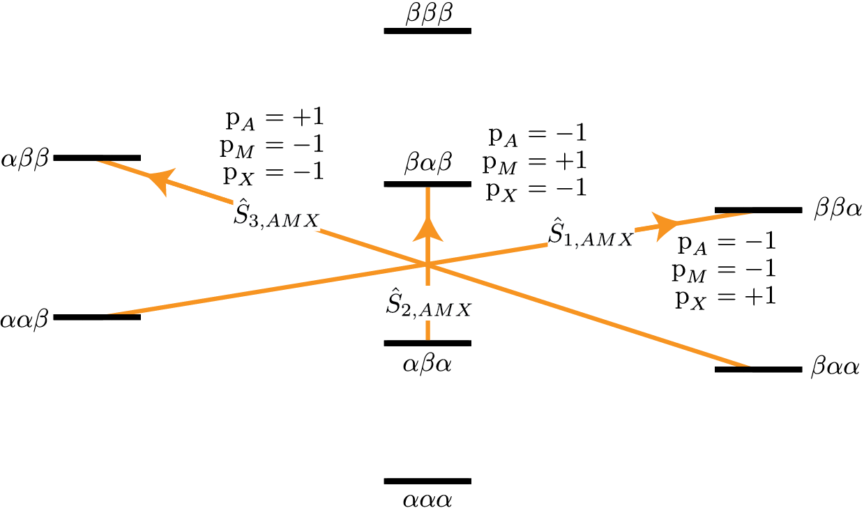
Figure 30 Energy level diagram for three coupled spin \(I=1/2\) nuclei. Arrows beginning at the initial state and end at the final state represent the three spin single-quantum transitions. Transitions are labeled with their corresponding single-spin \(\text{p}_i\) transition symmetry function values.
The code below will select these three-spin single-quantum transitions.
method = Method(
    channels=["1H"],
    magnetic_flux_density=9.4,  # in T
    spectral_dimensions=[
        SpectralDimension(
            count=16000,
            spectral_width=4000,  # in Hz
            reference_offset=1000,  # in Hz
            label="$^{1}$H frequency",
            events=[SpectralEvent(transition_queries=[{"ch1": {"P": [-1, -1, +1]}}])]
        )
    ],
)

sim = Simulator(spin_systems=[proton_system], methods=[method])
sim.run()
plt.figure(figsize=(10, 3))  # set the figure size
ax = plt.subplot(projection="csdm")
ax.plot(processor.apply_operations(dataset=sim.methods[0].simulation).real)
ax.invert_xaxis()  # reverse x-axis
plt.tight_layout()
plt.grid()
plt.show()

The assignment of transitions in the spectrum above, from left to right, are \(\hat{S}_{3,AMX}\), \(\hat{S}_{2,AMX}\), and \(\hat{S}_{1,AMX}\)
Again, combined with the three-site SpinSystem instance, the SymmetryQuery is expanded into the set of spin-system-specific symmetry queries illustrated in the table below.
Transitions |
\(\text{p}_A\) |
\(\text{p}_M\) |
\(\text{p}_X\) |
|---|---|---|---|
\(\hat{S}_{1,AMX}\) |
–1 |
+1 |
–1 |
\(\hat{S}_{2,AMX}\) |
–1 |
–1 |
+1 |
\(\hat{S}_{3,AMX}\) |
+1 |
–1 |
–1 |
from pprint import pprint
pprint(method.get_transition_pathways(proton_system))
[|0.5, -0.5, -0.5⟩⟨-0.5, 0.5, 0.5|, weight=(1+0j),
|-0.5, 0.5, -0.5⟩⟨0.5, -0.5, 0.5|, weight=(1+0j),
|-0.5, -0.5, 0.5⟩⟨0.5, 0.5, -0.5|, weight=(1+0j)]
As you can surmise from the examples, the attributes of SymmetryQuery, P and
D, holds a list of single-spin transition symmetry function values, and the
length of the list is the desired number of spins that are involved in the
transition.
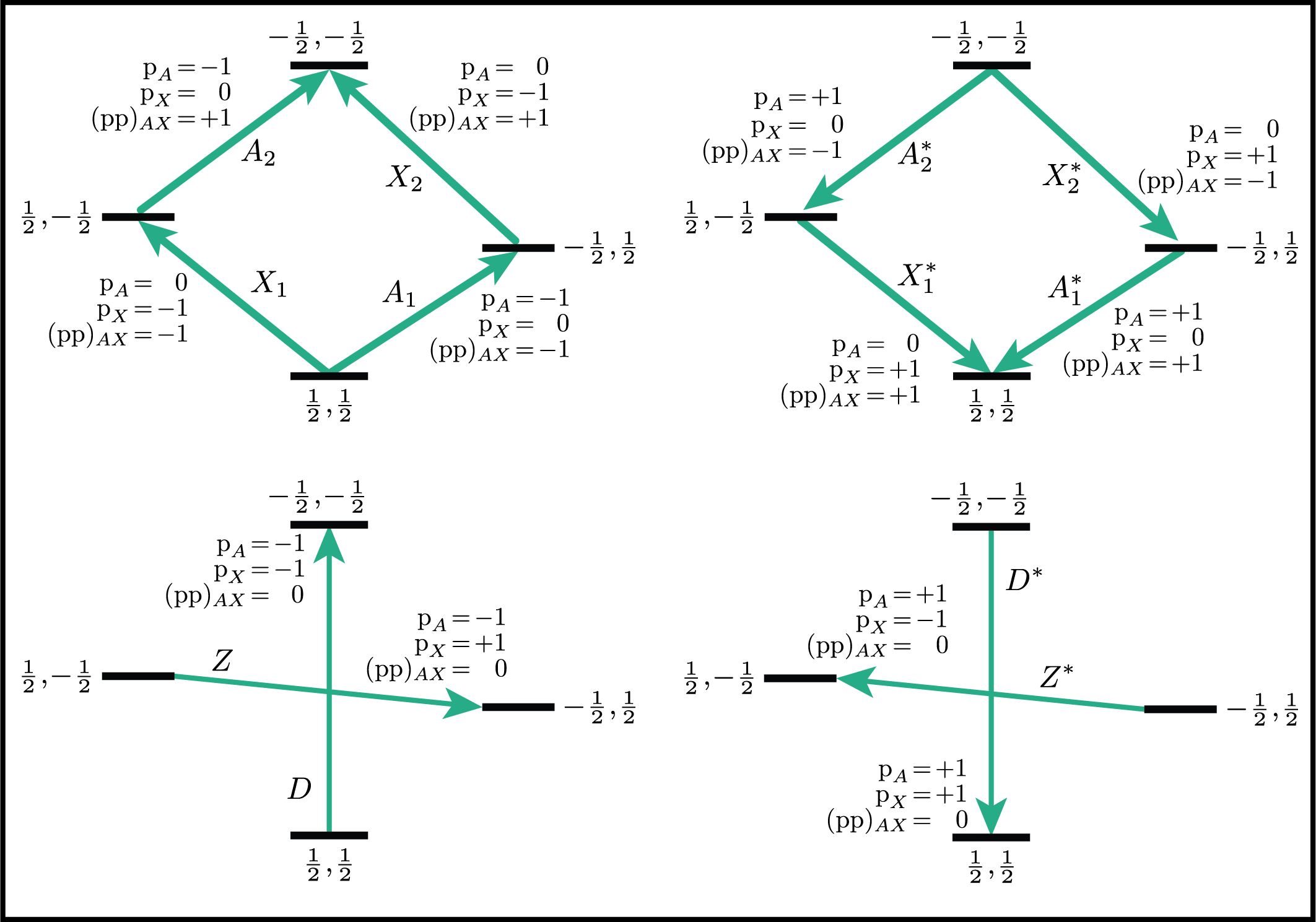
Heteronuclear multiple-spin transitions
How does D fit into the multi-site SymmetryQuery story? Consider the
case of two coupled hydrogens, except we replace one of the \(^1H\) with
\(^2H\). Let’s focus on the single-spin, single-quantum transitions, shown
below as \(\hat{A}_{1\pm}\) and \(\hat{A}_{2\pm}\) on the left, and the
two-spin triple-quantum transition, shown below as \(\hat{T}_{AX}\) on
the right.
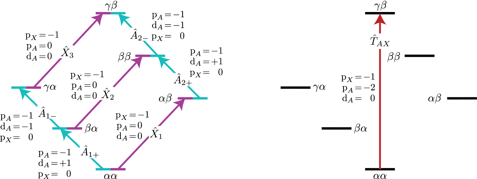
Figure 31 Energy level diagram for two coupled nuclei with spins \(I=1/2\) and \(I=1\). Arrows beginning at the initial state and ending at the final state represent the single-spin single-quantum transitions (left) and the three-spin triple-quantum transition. Transitions are labeled with their corresponding single-spin \(\text{p}_i\) transition symmetry function values.
from mrsimulator.spin_system.tensors import SymmetricTensor
import numpy as np

site_A = Site(
    isotope="2H",
    isotropic_chemical_shift=0.5,
    quadrupolar=SymmetricTensor(
        Cq=100000,  # in Hz
        eta=0.2,
        alpha=5 * np.pi / 180,
        beta=np.pi / 2,
        gamma=70 * np.pi / 180,
    ),
)
site_X = Site(isotope="1H", isotropic_chemical_shift=4.5)
sites = [site_A, site_X]
coupling_AX = Coupling(site_index=[0, 1], dipolar={"D": -20000})
couplings = [coupling_AX]
system_AX = SpinSystem(sites=sites, couplings=couplings)

methodAll1Q = Method(
    channels=["2H", "1H"],
    magnetic_flux_density=9.4,  # in T
    spectral_dimensions=[
        SpectralDimension(
            count=16000,
            spectral_width=200000,  # in Hz
            reference_offset=0,  # in Hz
            label="$^{2}$H frequency",
            events=[SpectralEvent(transition_queries=[{"ch1": {"P": [-1]}}])],
        )
    ],
)

methodHalf1Q = Method(
    channels=["2H", "1H"],
    magnetic_flux_density=9.4,  # in T
    spectral_dimensions=[
        SpectralDimension(
            count=16000,
            spectral_width=200000,  # in Hz
            reference_offset=0,  # in Hz
            label="$^{2}$H frequency",
            events=[SpectralEvent(transition_queries=[{"ch1": {"P": [-1], "D": [-1]}}])],
        )
    ],
)

method3Q = Method(
    channels=["2H", "1H"],
    magnetic_flux_density=9.4,  # in T
    spectral_dimensions=[
        SpectralDimension(
            count=16000,
            spectral_width=10000,  # in Hz
            reference_offset=5000,  # in Hz
            label="$^{2}$H frequency",
            events=[
                SpectralEvent(
                    transition_queries=[{"ch1": {"P": [-2]}, "ch2": {"P": [-1]}}]
                )
            ],
        )
    ],
)
processor = sp.SignalProcessor(
    operations=[sp.IFFT(), sp.apodization.Gaussian(FWHM="100 Hz"), sp.FFT()]
)

sim = Simulator(spin_systems=[system_AX], methods=[methodAll1Q, methodHalf1Q, method3Q])
sim.config.integration_volume = "hemisphere"
sim.run()
fig, ax = plt.subplots(1, 2, figsize=(10, 3.5), subplot_kw={"projection": "csdm"}, sharey=True)
ax[0].plot(processor.apply_operations(dataset=sim.methods[0].simulation).real)
ax[0].set_title("Full Single-Quantum Spectrum")
ax[0].grid()
ax[0].invert_xaxis()  # reverse x-axis
ax[1].plot(processor.apply_operations(dataset=sim.methods[1].simulation).real)
ax[1].set_title("Half Single-Quantum Spectrum")
ax[1].grid()
ax[1].invert_xaxis()  # reverse x-axis
plt.tight_layout()
plt.show()
The deuterium spectrum of a static-polycrystalline sample is shown on the left for all single-spin single-quantum transitions on deuterium, \(\hat{A}_{1\pm}\) and \(\hat{A}_{2\pm}\). The spectrum on the right is for half of the single-spin single-quantum transitions on deuterium: \(\hat{A}_{1-}\) and \(\hat{A}_{2-}\).
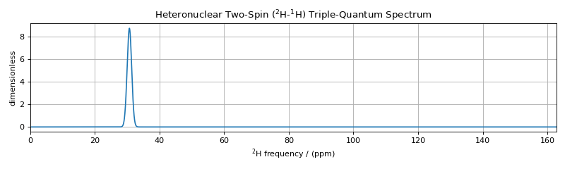
plt.figure(figsize=(10, 3))  # set the figure size
ax = plt.subplot(projection="csdm")
ax.set_title("Heteronuclear Two-Spin ($^2$H-$^1$H) Triple-Quantum Spectrum")
ax.plot(processor.apply_operations(dataset=sim.methods[2].simulation).real)
plt.tight_layout()
plt.grid()
plt.show()

Transitions |
\(\text{p}_A\) |
\(\text{d}_A\) |
\(\text{p}_X\) |
|---|---|---|---|
\(\hat{T}_{AX}\) |
–2 |
0 |
–1 |
The single transition in the heteronuclear two-spin (\(^2\text{H}\)-\(^1\text{H}\)) triple-quantum spectrum is unaffected by the dipolar and quadrupolar frequency anisotropies.
Frequency Contributions
The NMR frequency, \(\Omega(\Theta,i,j)\), of an \(i \rightarrow j\) transition between the eigenstates of the stationary-state semi-classical Hamiltonian in a sample with a lattice spatial orientation, \(\Theta\), can be written as a sum of components,
with each component, \(\Omega_k(\Theta,i,j)\), separated into three parts:
where \({\xi}^{(k)}_\ell(i,j)\) are the spin transition symmetry functions described earlier, \({\Xi}^{(k)}_L(\Theta)\) are the spatial symmetry functions, and \(\omega_k\) gives the size of the kth frequency component. The experimentalist indirectly influences a frequency component \(\Omega_k\) by direct manipulation of the quantum transition, \(i \rightarrow j\), and the spatial orientation, \(\Theta\), of the sample.
The function symbol \(\Xi_\ell(\Theta)\) is replaced with the upper-case symbols \(\mathbb{S}\), \(\mathbb{P}(\Theta)\), \(\mathbb{D}(\Theta)\), \(\mathbb{F}(\Theta)\), \(\mathbb{G}(\Theta)\), \(\ldots\), i.e., following the spectroscopic sub-shell letter designations for \(L\). Consult the Symmetry Pathways paper for more details on the form of the spatial symmetry functions. In short, the \(\mathbb{S}\) function is independent of sample orientation, i.e., it will appear in all isotropic frequency contributions. The \(\mathbb{D}(\Theta)\) function has a second-rank dependence on sample orientation, and can be averaged away with fast magic-angle spinning, i.e., spinning about an angle, \(\theta_R\), that is the root of the second-rank Legendre polynomial \(P_2(\cos \theta_R)\). The other spatial symmetry functions are removed by spinning the sample about the corresponding root of the \(L^\text{th}\)-rank Legendre polynomial \(P_L(\cos \theta_R)\)
Note
For 2nd-order quadrupolar coupling contributions, it is convenient to define “hybrid” spin transition functions as linear combinations of the spin transition functions
These transition symmetry functions play an essential role in evaluating the
individual frequency contributions to the overall transition frequency, given in
the table below and in
FrequencyEnum(). They also aid in
pulse sequence design by identifying how different frequency contributions
refocus through the transition pathways.
For a summary on echo symmetry classification in NMR, click on the disclosure button below.
Echo Symmetry Classification
Note
The well-known Hahn-echo can occur whenever the \(p_I\) values of transitions in a transition pathway change sign. This is because the changing sign of \(p_I\) leads to a sign change for every \(p_I\)-dependent transition frequency contribution. Thus, a Hahn echo forms whenever
assuming a frequency contribution’s spatial symmetry function, \({\Xi}\), remains constant during this period. As seen in the table in the Frequency Contributions table, sign changes in other symmetry functions can also lead to corresponding sign changes for dependent frequency contributions. Thus, a problem with showing only the \(p_I\) symmetry pathway for an NMR method is that it does not explain the formation of other classes of echoes that result when other symmetry functions change sign in a transition pathway. To fully understand when and which frequency contributions refocus into echoes, we must follow all relevant spatial, transition, or spatial-transition product symmetries through an NMR experiment. Thus, we generally classify echoes that refocus during a time interval as a transition symmetry echo (at constant \({\Xi}_k\)) when
and as a spatial symmetry echo (at constant \({\xi}_k\)) when
and as a spatial-transition symmetry product echo when
Within the class of transition echoes, we find subclasses such as \(\text{p}\) echoes, which include the Hahn echo and the stimulated echo; \(\text{d}\) echoes, which include the solid echo and Solomon echoes, \(\text{c}_4\) echoes, used in MQ-MAS and Satellite-Transition Magic-Angle Spinning (ST-MAS); \(\text{c}_2\) echoes, used in Correlation Of Anisotropies Separated Through Echo Refocusing (COASTER); and \(\text{c}_0\) echoes, used in Multiple-Quantum DOuble Rotation (MQ-DOR).
Within the class of spatial echoes, we find subclasses such as \(\mathbb{D}\) rotary echoes, which occur during sample rotation, and \(\mathbb{D}_0\) and \(\mathbb{G}_0\) echoes, which are designed to occur simultaneously during the Dynamic-Angle Spinning (DAS) experiment.
Interactions |
perturbation
order
|
anisotropy
rank
|
|
Expression |
|---|---|---|---|---|
shielding |
1st |
0th |
|
\({\boldsymbol \Delta}_{0}^{\{\sigma\}} \mathbb{p}_I\) |
shielding |
1st |
2nd |
|
\({\boldsymbol \Delta}_{2}^{\{\sigma\}} \mathbb{p}_I\) |
weak J |
1st |
0th |
|
\({\boldsymbol \Delta}_{0}^{\{J\}} (\mathbb{pp})_{IS}\) |
weak J |
1st |
2nd |
|
\({\boldsymbol \Delta}_{2}^{\{J\}} \cdot (\mathbb{pp})_{IS}\) |
weak dipolar |
1st |
2nd |
|
\({\boldsymbol \Delta}_{2}^{\{d_{IS}\}} (\mathbb{pp})_{IS}\) |
quadrupolar |
1st |
2nd |
|
\({\boldsymbol \Delta}_{2}^{\{q\}} \mathbb{d}_I\) |
quadrupolar |
2nd |
0th |
|
\({\boldsymbol \Delta}_{0}^{\{qq\}} \mathbb{c}_0\) |
quadrupolar |
2nd |
2nd |
|
\({\boldsymbol \Delta}_{2}^{\{qq\}} \mathbb{c}_2\) |
quadrupolar |
2nd |
4th |
|
\({\boldsymbol \Delta}_{4}^{\{qq\}} \mathbb{c}_4\) |
quadrupolar-shielding |
2nd |
0th |
|
\({\boldsymbol \Delta}_{0}^{\{\sigma q\}} \mathbb{d}_I\) |
quadrupolar-shielding |
2nd |
2nd |
|
\({\boldsymbol \Delta}_{2}^{\{\sigma q\}} \mathbb{d}_I\) |
quadrupolar-shielding |
2nd |
4th |
|
\({\boldsymbol \Delta}_{4}^{\{\sigma q\}} \mathbb{d}_I\) |
quadrupolar-weak dipole |
2nd |
0th |
|
\({\boldsymbol \Delta}_{0}^{\{d q\}} (\mathbb{d}\mathbb{p})_{IS}\) |
quadrupolar-weak dipole |
2nd |
2nd |
|
\({\boldsymbol \Delta}_{2}^{\{d q\}} (\mathbb{d}\mathbb{p})_{IS}\) |
quadrupolar-weak dipole |
2nd |
4th |
|
\({\boldsymbol \Delta}_{4}^{\{d q\}} (\mathbb{d}\mathbb{p})_{IS}\) |
quadrupolar-weak J |
2nd |
0th |
|
\({\boldsymbol \Delta}_{0}^{\{J q\}} (\mathbb{d}\mathbb{p})_{IS}\) |
quadrupolar-weak J |
2nd |
2nd |
|
\({\boldsymbol \Delta}_{2}^{\{J q\}} (\mathbb{d}\mathbb{p})_{IS}\) |
quadrupolar-weak J |
2nd |
4th |
|
\({\boldsymbol \Delta}_{4}^{\{J q\}} (\mathbb{d}\mathbb{p})_{IS}\) |
Affine Transformations
The ability to refocus different spatial and transition symmetries into echoes with different paths in time-resolved NMR experiments create opportunities for generating multi-dimensional spectra that correlate different interactions. These spectra can be made easier to interpret through similarity transformations. Most similarity transformations in NMR are affine transformations, as they preserve the colinearity of points and ratios of distances. Essential in any similarity transformation is whether to implement the transformation actively or passively. Active transformations change the appearance of the signal while leaving the coordinate system unchanged, whereas passive transformations leave the appearance of the signal unchanged while changing the coordinate system. Both active and passive transformations are used extensively in NMR.
The general form of the affine transformation of a n-dimensional spectrum is
In the two-dimensional case, this is given by
Note
For the multiple-quantum MAS experiment, a shear and scale transformation is often applied to the spectrum to create a 2D spectrum correlating the MQ-MAS isotropic frequency to the anisotropic central transition frequency. This correlation can be achieved by adding an affine matrix to the method.
For 3Q-MAS on a spin \(I=3/2\) nucleus, where the shear factor is \(\kappa^{(\omega_2)} = 21/27\), the affine matrix giving the appropriate shear and scale transformation is given by
After the affine transformation, the position of the resonance in the isotropic projection is a weighted average of the multiple quantum and central transition isotropic frequencies given by
If the spectrum is to be referenced to a frequency other than the RF carrier frequency (i.e. zero is not defined in the middle of the spectrum), then the reference offset used in the single-quantum dimension must be multiplied by a factor of \({\left({\text{p}_I^{[1]}}/{\text{p}_I^{[2]}} + |\kappa^{(\omega_1)}| \right)/(1+ |\kappa^{(\omega_1)}| )}\) when used in the isotropic dimension.
See the “Symmetry Pathways in Solid-State NMR” paper for a more detailed discussion on affine transformations in NMR.
In the code below, the 3Q-MAS method described earlier is modified to include an affine matrix to perform this shear transformation.
my_sheared_mqmas = Method(
    channels=["87Rb"],
    magnetic_flux_density=9.4,
    rotor_frequency=np.inf,  # in Hz (here, set to infinity)
    spectral_dimensions=[
        SpectralDimension(
            count=128,
            spectral_width=6e3,  # in Hz
            reference_offset=-9e3,  # in Hz
            label="3Q-MAS isotropic dimension",
            events=[
                SpectralEvent(transition_queries=[{"ch1": {"P": [-3], "D": [0]}}])
            ],
        ),
        SpectralDimension(
            count=256,
            spectral_width=6e3,  # in Hz
            reference_offset=-5e3,  # in Hz
            label="Central Transition Frequency",
            events=[
                SpectralEvent(transition_queries=[{"ch1": {"P": [-1], "D": [0]}}])
            ],
        ),
    ],
    affine_matrix=[[9 / 16, 7 / 16], [0, 1]],
)

sim = Simulator(spin_systems=RbNO3_spin_systems, methods=[my_sheared_mqmas])
sim.run()

dataset = gauss_convolve.apply_operations(dataset=sim.methods[0].simulation)
plt.figure(figsize=(4, 3))
ax = plt.subplot(projection="csdm")
cb = ax.imshow(dataset.real / dataset.real.max(), aspect="auto", cmap="gist_ncar_r")
plt.colorbar(cb)
ax.invert_xaxis()
ax.invert_yaxis()
plt.tight_layout()
plt.show()

Note
For MQ-MAS, a second shear and scale can be applied to remove isotropic chemical shift component along the \(\Omega^{[2]''}\) axis. For a spin \(I=3/2\) nucleus, with a second shear factor of \(\kappa^{(\omega_1)} = - 8/17\), the affine matrix is given by
and the product of the two affine transformations is
Below is the code for simulating a 3Q-MAS spectrum with a double shear transformation.
my_twice_sheared_mqmas = Method(
    channels=["87Rb"],
    magnetic_flux_density=9.4,
    rotor_frequency=np.inf,  # in Hz (here, set to infinity)
    spectral_dimensions=[
        SpectralDimension(
            count=128,
            spectral_width=6e3,  # in Hz
            reference_offset=-9e3,  # in Hz
            label="3Q-MAS isotropic dimension",
            events=[
                SpectralEvent(transition_queries=[{"ch1": {"P": [-3], "D": [0]}}])
            ],
        ),
        SpectralDimension(
            count=256,
            spectral_width=6e3,  # in Hz
            reference_offset=0,  # in Hz
            label="CT Quad-Only Frequency",
            events=[
                SpectralEvent(transition_queries=[{"ch1": {"P": [-1], "D": [0]}}])
            ],
        ),
    ],
    affine_matrix=[[9 / 16, 7 / 16], [-9 / 50, 27 / 50]],
)

sim = Simulator(spin_systems=RbNO3_spin_systems, methods=[my_twice_sheared_mqmas])
sim.run()

dataset = gauss_convolve.apply_operations(dataset=sim.methods[0].simulation)
plt.figure(figsize=(4, 3))
ax = plt.subplot(projection="csdm")
cb = ax.imshow(dataset.real / dataset.real.max(), aspect="auto", cmap="gist_ncar_r")
plt.colorbar(cb)
ax.invert_xaxis()
ax.invert_yaxis()
plt.tight_layout()
plt.show()

Average Frequency & Multiple Events
To illustrate the versatility of the Method class, we can also design an MQ-MAS method that correlates the isotropic MQ-MAS frequency to the central transition without the need for an affine transformation. Recall that the 3Q-MAS isotropic frequency on spin \(I=3/2\) is given by
As we saw at the beginning of this section, the first spectral dimension derives its average frequency, \(\overline{\Omega}_1\), from a weighted average of multiple transition frequencies. Thus, this weighted average frequency can be obtained through the use of multiple SpectralEvent instances in the SpectralDimension associated with the isotropic dimension, as shown in the code below.
my_three_event_mqmas = Method(
    channels=["87Rb"],
    magnetic_flux_density=9.4,
    rotor_frequency=np.inf,  # in Hz (here, set to infinity)
    spectral_dimensions=[
        SpectralDimension(
            count=128,
            spectral_width=6e3,  # in Hz
            reference_offset=-9e3,  # in Hz
            label="3Q-MAS isotropic dimension",
            events=[
                SpectralEvent(
                    fraction=9 / 16, transition_queries=[{"ch1": {"P": [-3], "D": [0]}}]
                ),
                SpectralEvent(
                    fraction=7 / 16, transition_queries=[{"ch1": {"P": [-1], "D": [0]}}]
                ),
            ],
        ),
        SpectralDimension(
            count=256,
            spectral_width=6e3,  # in Hz
            reference_offset=-5e3,  # in Hz
            label="Central Transition Frequency",
            events=[
                SpectralEvent(transition_queries=[{"ch1": {"P": [-1], "D": [0]}}])
            ],
        ),
    ],
)

sim = Simulator(spin_systems=RbNO3_spin_systems, methods=[my_three_event_mqmas])
sim.run()

dataset = gauss_convolve.apply_operations(dataset=sim.methods[0].simulation)
plt.figure(figsize=(4, 3))
ax = plt.subplot(projection="csdm")
cb = ax.imshow(dataset.real / dataset.real.max(), aspect="auto", cmap="gist_ncar_r")
plt.colorbar(cb)
ax.invert_xaxis()
ax.invert_yaxis()
plt.tight_layout()
plt.show()

We could apply an affine transformation to remove the isotropic chemical shift
from the central transition (horizontal) dimension. If you go back to the
previous discussion, you will find that the required value for the
affine_matrix in the Method instance to do this shear is given by
affine_matrix=[[1,0],[-8/25, 17/25]]
RotationEvent
The amplitude of a transition pathway signal derives from the product of mixing amplitudes associated with each transfer between transitions in a transition pathway, e.g.,
Here, \(a_{0A}\) is the amplitude of the initial \(\hat{t}_A\) transition, \(a_{AB}\) is the mixing amplitude for the transfer from \(\hat{t}_A\) to \(\hat{t}_B\), \(a_{BC}\) is the mixing amplitude for the transfer from \(\hat{t}_B\) to \(\hat{t}_C\), and so on. The growing product \((a_{0A}a_{AB}a_{BC} \cdots)\) is the transition pathway amplitude. Eliminating a transition with a TransitionQuery in a spectral or delay event sets the eliminated transition’s pathway amplitude to zero, i.e., it prunes that transition pathway branch.
Default Total Mixing between Adjacent Spectral or Delay Events
In previous discussions, we did not mention the efficiency of transfer between selected transitions in adjacent FreeEvent instances. This is because, as default behavior, MRSimulator does a total mixing, i.e., connects all selected transitions in the two adjacent FreeEvent instances. In other words, if the first of two adjacent FreeEvent instances has three selected transitions and the second has two selected transitions, then MRSimulator will make \(3 \times 2 = 6\) connections, i.e., six transition pathways passing from the first to second SpectralEvent instances.
Additionally, this total mixing assumes that every connection has a mixing amplitude of 1. This is unrealistic, but if used correctly gives a significant speed-up in the simulation by avoiding the need to calculate mixing amplitudes.
Warning
The use of total mixing, i.e., the default mixing, can complicate the comparison of integrated intensities between different methods, depending on the selected transition pathways.
However, when multiple transition pathways are present in a method, you may need more accurate mixing amplitudes when connecting selected transitions of adjacent events. You may also need to prevent the undesired mixing of specific transitions between two adjacent events. As described below, you can avoid a total mixing event by inserting the RotationEvent instance with Rotation instances assigned to different channels.
Rotation
A rotation of \(\theta\) about an axis defined by \(\phi\) in the \(x\)-\(y\) plane on a selected transition, \(\ketbra{I, m_f}{I, m_i}\), in a spectral or delay event transfers it to all selected transitions, \(\ketbra{I,m_f'}{I,m_i'}\) in the next spectral or delay event, according to
where \(\Delta p_I = p_I' - p_I\). From this expression, we obtain the complex mixing amplitude from \(\ketbra{I, m_f}{I, m_i}\) to \(\ketbra{I, m_f'}{I, m_i'}\) due to a rotation to be
From this expression, we note a few interesting and useful cases. One is the coherence transfer under a \(\pi\) rotation, given by
That is, a \(\pi\) rotation can make only one connection between transitions in adjacent events. It is also a special connection because the \(\text{p}_I\) transition symmetry value for the two transitions are equal but opposite in sign. Additionally, the \(\text{d}_I\) transition symmetry remains unchanged (\(\Delta \text{d}_I = 0\)) for the two transitions. (In fact, this behavior under a \(\pi\) rotation is generally true for odd (\(\text{p}_I, \text{f}_I, \ldots)\) and even (\(\text{d}_I, \text{g}_I, \ldots)\) rank spin transition symmetry functions.)
Another interesting result is that, while a rotation can transfer a transition into many other transitions, the \(\text{d}_I\) transition symmetry value cannot remain unchanged (\(\Delta \text{d}_I \neq 0\)) between two connected transitions under a \(\pi/2\) rotation.
Finally, another useful result is
While it’s unsurprising that a rotation through an angle of zero does nothing to the transition, this turns out to help act as the opposite of a total mixing event, i.e., a no mixing event. This can be implemented with the code below.
from mrsimulator.method import RotationEvent

RotationEvent()  # empty instance defaults to a zero rotation on all channels.
The RotationEvent instance holds the rotation details in a RotationEvent instance as
a Rotation instance associated with a channels attribute. This is
illustrated in the sample code below.
import numpy as np
from mrsimulator.method.query import Rotation
rot_query_90 = Rotation(angle=np.pi/2, phase=0)
rot_query_180 = Rotation(angle=np.pi, phase=0)
rot_mixing = RotationEvent(
        ch1=rot_query_90,
        ch2=rot_query_180
    )
p and d Echoes on Deuterium
Here, we examine two examples in a deuterium spin system that illustrate the importance of echo classification in understanding how transition-frequency contributions can be eliminated or separated based on their dependence on different transition symmetry functions.
First, we implement two Method instances that follow the design of two experimental pulse sequences. In this effort, we use Rotation instances to select the desired transition pathways and obtain spectra with the desired average frequencies. Then, we implement two simpler Method instances that produce identical spectra and illustrate how frequency contributions can be used to reduce the number of events needed in a custom method.
Consider the Hahn and Solid Echo pulse sequences on the left and right, respectively.
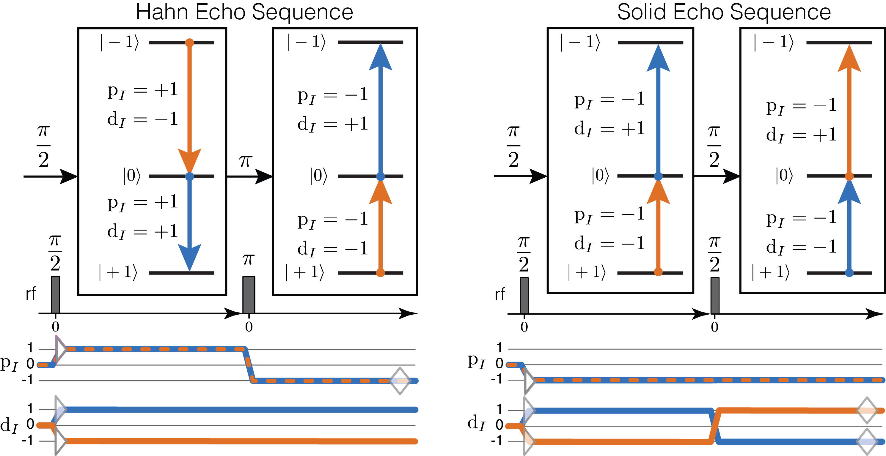
Figure 32 Hahn Echo (left) and Solid-Echo (right) pulse sequences. Above each sequence, on the energy level diagram are the corresponding two transition pathways indicated with blue and orange arrows. Transitions are labeled with their corresponding \(\text{p}_I\) and \(\text{d}_I\) transition symmetry function values. Below each sequence are the corresponding transition symmetry pathways, also in blue and orange.
The Hahn Echo sequence, with \(\pi/2-\tau-\pi-t\rightarrow\), leads to the formation of a \(\text{p}_I\) echo at \(t = \tau\). The two transition pathways created by this experiment on a deuterium nucleus are illustrated beneath the sequence. Remember that a \(\pi\) rotation is special because it connects transitions with equal but opposite signs of \(\text{p}_I\) while \(\text{d}_I\) remains invariant.
The Solid Echo sequence, with \(\pi/2-\tau-\pi/2-t\rightarrow\), leads to the formation of a \(\text{d}_I\) echo at \(t = \tau\). The two transition pathways created by this experiment on a deuterium nucleus are illustrated beneath the sequence. Here, also recall that the \(\text{d}_I\) transition symmetry value cannot remain unchanged (\(\Delta \text{d}_I \neq 0\)) between two connected transitions under a \(\pi/2\) rotation.
Below are two custom Method instances for simulating the Hahn and Solid Echo experiments. There is only one SpectralDimension instance in each method, and the average frequency during each spectral dimension is derived from equal fractions of two SpectralEvent instances. Between these two SpectralEvent instances is a RotationEvent with a Rotation instance. The Rotation instance is created with a \(\pi\) rotation in the Hahn Echo method and a \(\pi/2\) rotation in the Solid Echo method.
Note
The transition_queries attribute of SpectralEvent holds a list of
TransitionQuery instances. Each TransitionQuery in the list applies to
the full set of transitions in the spin system. The union of these transition
subsets becomes the final set of selected transitions during the
SpectralEvent.
We use the deuterium Site defined earlier in this document.
deuterium = Site(
    isotope="2H",
    isotropic_chemical_shift=10,  # in ppm
    shielding_symmetric={"zeta": -80, "eta": 0.25},  # zeta in ppm
    quadrupolar={"Cq": 10e3, "eta": 0.0, "alpha": 0, "beta": np.pi / 2, "gamma": 0},
)
deuterium_system = SpinSystem(sites=[deuterium])

hahn_echo = Method(
    channels=["2H"],
    magnetic_flux_density=9.4,  # in T
    rotor_angle=0,  # in rads
    spectral_dimensions=[
        SpectralDimension(
            count=512,
            spectral_width=2e4,  # in Hz
            events=[
                SpectralEvent(
                    fraction=0.5,
                    transition_queries=[
                        {"ch1": {"P": [1], "D": [1]}},
                        {"ch1": {"P": [1], "D": [-1]}},
                    ],
                ),
                RotationEvent(ch1={"angle": 3.141592, "phase": 0}),
                SpectralEvent(
                    fraction=0.5,
                    transition_queries=[
                        {"ch1": {"P": [-1], "D": [1]}},
                        {"ch1": {"P": [-1], "D": [-1]}},
                    ],
                ),
            ],
        )
    ],
)

solid_echo = Method(
    channels=["2H"],
    magnetic_flux_density=9.4,  # in T
    rotor_angle=0,  # in rads
    spectral_dimensions=[
        SpectralDimension(
            count=512,
            spectral_width=2e4,  # in Hz
            events=[
                SpectralEvent(
                    fraction=0.5,
                    transition_queries=[
                        {"ch1": {"P": [-1], "D": [1]}},
                        {"ch1": {"P": [-1], "D": [-1]}},
                    ],
                ),
                RotationEvent(ch1={"angle": 3.141592 / 2, "phase": 0}),
                SpectralEvent(
                    fraction=0.5,
                    transition_queries=[
                        {"ch1": {"P": [-1], "D": [1]}},
                        {"ch1": {"P": [-1], "D": [-1]}},
                    ],
                ),
            ],
        )
    ],
)
We can check the resulting transition pathways using these TransitionQuery instances with the
code below for the hahn_echo method,
from pprint import pprint
pprint(hahn_echo.get_transition_pathways(deuterium_system))
[|1.0⟩⟨0.0| ⟶ |-1.0⟩⟨0.0|, weight=(1+0j)
 |0.0⟩⟨-1.0| ⟶ |0.0⟩⟨1.0|, weight=(1+0j)]
and for the solid_echo method with the code below.
pprint(solid_echo.get_transition_pathways(deuterium_system))
[|-1.0⟩⟨0.0| ⟶ |0.0⟩⟨1.0|, weight=(0.5+0j)
 |0.0⟩⟨1.0| ⟶ |-1.0⟩⟨0.0|, weight=(0.5+0j)]
Notice that the weights of the transition pathways in the solid-echo method are half of those in the Hahn-echo method. This is because the \(\pi\) pulse in the Hahn-echo method gives perfect transfer between the two transitions in the adjacent FreeEvent instances. In contrast, while the \(\pi/2\) pulse in the solid-echo method prevents the undesired transition pathways with \(\Delta \text{d}_I = 0\), it also connects the selected transitions during the first spectral event to undesired transitions in the second spectral event, which are eliminated by its symmetry query.
Next, we simulate both methods and perform a Gaussian line shape convolution on each output spectrum, and plot the datasets.
sim = Simulator(spin_systems=[deuterium_system], methods=[hahn_echo, solid_echo])
sim.run()

processor = sp.SignalProcessor(
    operations=[
        sp.IFFT(),
        sp.apodization.Gaussian(FWHM="100 Hz"),
        sp.FFT(),
    ]
)
hahn_dataset = processor.apply_operations(dataset=sim.methods[0].simulation)
solid_dataset = processor.apply_operations(dataset=sim.methods[1].simulation)
fig, ax = plt.subplots(1, 2, subplot_kw={"projection": "csdm"}, figsize=[8.5, 3])
ax[0].set_title("Hahn-Echo Spectrum")
ax[0].plot(hahn_dataset.real)
ax[0].invert_xaxis()
ax[0].grid()
ax[1].set_title("Solid-Echo Spectrum")
ax[1].plot(solid_dataset.real)
ax[1].invert_xaxis()
ax[1].grid()
plt.tight_layout()
plt.show()
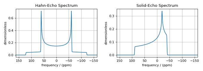
In the Hahn-echo spectrum, the \(\text{p}_I\)-dependent frequency contributions (i.e., the shielding contributions) were averaged to zero, leaving only the \(\text{d}_I\)-dependent frequency contributions (i.e., the first-order quadrupolar contribution). Conversely, in the solid-echo spectrum, the \(\text{d}_I\)-dependent frequency contributions (i.e., the first-order quadrupolar contribution) were averaged to zero, leaving only the \(\text{p}_I\)-dependent frequency contributions (i.e., the shielding contributions).
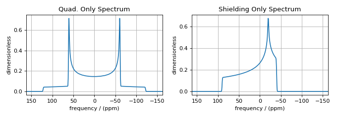
While these two examples nicely illustrate numerous important concepts for
building custom methods, it should also be noted that identical spectra could
have been obtained with a simpler custom method that used the freq_contrib
to only select the desired frequency contributions. The code for these two methods
is illustrated below.
quad_only = Method(
    channels=["2H"],
    magnetic_flux_density=9.4,  # in T
    spectral_dimensions=[
        SpectralDimension(
            count=512,
            spectral_width=2e4,  # in Hz
            events=[
                SpectralEvent(
                    transition_queries=[{"ch1": {"P": [-1]}}],
                    freq_contrib=["Quad1_2"]
                )
            ],
        )
    ],
)

shielding_only = Method(
    channels=["2H"],
    magnetic_flux_density=9.4,  # in T
    spectral_dimensions=[
        SpectralDimension(
            count=512,
            spectral_width=2e4,  # in Hz
            events=[
                SpectralEvent(
                    transition_queries=[{"ch1": {"P": [-1]}}],
                    freq_contrib=["Shielding1_0", "Shielding1_2"],
                )
            ],
        )
    ],
)

sim = Simulator()
sim.spin_systems = [SpinSystem(sites=[deuterium])]
sim.methods = [quad_only, shielding_only]
sim.run()

processor = sp.SignalProcessor(
    operations=[
        sp.IFFT(),
        sp.apodization.Gaussian(FWHM="100 Hz"),
        sp.FFT(),
    ]
)
quad_only_dataset = processor.apply_operations(dataset=sim.methods[0].simulation)
shielding_only_dataset = processor.apply_operations(dataset=sim.methods[1].simulation)
fig, ax = plt.subplots(1, 2, subplot_kw={"projection": "csdm"}, figsize=[8.5, 3])
ax[0].set_title("Quad. Only Spectrum")
ax[0].plot(quad_only_dataset.real)
ax[0].invert_xaxis()
ax[0].grid()
ax[1].set_title("Shielding Only Spectrum")
ax[1].plot(shielding_only_dataset.real)
ax[1].invert_xaxis()
ax[1].grid()
plt.tight_layout()
plt.show()
Note
mrsimulator also includes shortcuts for addressing groups of frequency
contributions together. For example, the shielding_only method could
have selected all shielding contributions by using
freq_contrib=["Shielding"] which expands to zeroth- and second-rank shielding.
A complete list of shortcuts are listed in FrequencyEnum.
Origin and Reference Offset
SpectralDimension() has additional
attributes that have already been discussed in earlier sections of the documentation.
Notably, origin_offset is important for converting the frequency coordinate into
a dimensionless frequency ratio coordinate. For spectra where all the spectral dimensions are associated with single-quantum transitions on a single isotope, the convention is to define
the origin_offset as the NMR spectrometer frequency of the primary reference for a given isotope. Thus, given the frequency coordinate, \({X}\), the corresponding
dimensionless-frequency ratio follows,
The reference_offset, \(b_k\), is then defined as the offset in hertz between
the primary reference frequency and the center frequency of the spectrum.
In the case of multiple quantum dimensions, however, there appear
to be no formal conventions for defining origin_offset and reference_offset.
Attribute Summaries
Attribute Name |
Type |
Description |
|---|---|---|
channels |
|
A required list of isotopes given as strings over which the given method applies.
For example, |
magnetic_flux_density |
|
An optional float describing the macroscopic magnetic flux density of the applied
external magnetic field in tesla. For example, |
rotor_frequency |
|
An optional float describing the sample rotation frequency in Hz. For example, |
rotor_angle |
|
An optional float describing the angle between the sample rotation axis and the external
magnetic field in radians. The default value is the magic angle,
|
spectral_dimensions |
|
A list of SpectralDimension instances describing the spectral dimensions for the method. |
affine_matrix |
|
An optional ( |
simulation |
CSDM instance |
A CSDM instance representing the spectrum simulated by the method. By default, the value is
|
experiment |
CSDM instance |
An optional CSDM instance holding an experimental measurement of the method. The default
value is |
Attribute Name |
Type |
Description |
|---|---|---|
count |
|
An optional integer representing the number of points, \(N\), along the spectroscopic
dimension. For example, |
spectral_width |
|
An optional float representing the width, \(\Delta x\), of the spectroscopic dimension
in Hz. For example, |
reference_offset |
|
An optional float representing the reference offset, \(x_0\), of the spectroscopic
dimension in Hz. For example, |
origin_offset |
|
An optional float representing the origin offset, or primary reference frequency, along the
spectroscopic dimension in units of Hz. The default value is |
events |
|
An optional list of Events used to emulate an experiment. The default value is an empty list. |
Attribute Name |
Type |
Description |
|---|---|---|
magnetic_flux_density |
|
An optional float describing the macroscopic magnetic flux density of the applied
external magnetic field in Tesla. For example, |
rotor_angle |
|
An optional float describing the angle between the sample rotation axis and the external
magnetic field in radians. The default is |
rotor_frequency |
|
An optional float describing the sample rotation frequency in Hz. For example, |
freq_contrib |
|
An optional list of FrequencyEnum (list of allowed strings) selecting which
contributions to include when calculating a transition frequency. For example,
|
transition_queries |
|
An optional |
Attribute Name |
Type |
Description |
|---|---|---|
\(\text{ch}i\) |
|
A |