Wollastonite, 29Si (I=1/2)

29Si (I=1/2) spinning sideband simulation.

Wollastonite is a high-temperature calcium-silicate, \(\beta−\text{Ca}_3\text{Si}_3\text{O}_9\), with three distinct \(^{29}\text{Si}\) sites. The \(^{29}\text{Si}\) tensor parameters were obtained from Hansen et. al. 1

import matplotlib as mpl
import matplotlib.pyplot as plt
import mrsimulator.signal_processing as sp
import mrsimulator.signal_processing.apodization as apo
from mrsimulator import Simulator, SpinSystem, Site
from mrsimulator.methods import BlochDecaySpectrum

# global plot configuration
mpl.rcParams["figure.figsize"] = [4.5, 3.0]

Step 1: Create the sites.

S29_1 = Site(
    isotope="29Si",
    isotropic_chemical_shift=-89.0,  # in ppm
    shielding_symmetric={"zeta": 59.8, "eta": 0.62},  # zeta in ppm
)
S29_2 = Site(
    isotope="29Si",
    isotropic_chemical_shift=-89.5,  # in ppm
    shielding_symmetric={"zeta": 52.1, "eta": 0.68},  # zeta in ppm
)
S29_3 = Site(
    isotope="29Si",
    isotropic_chemical_shift=-87.8,  # in ppm
    shielding_symmetric={"zeta": 69.4, "eta": 0.60},  # zeta in ppm
)

sites = [S29_1, S29_2, S29_3]  # all sites

Step 2: Create the spin systems from these sites. Again, we create three single-site spin systems for better performance.

spin_systems = [SpinSystem(sites=[s]) for s in sites]

Step 3: Create a Bloch decay spectrum method.

method = BlochDecaySpectrum(
    channels=["29Si"],
    magnetic_flux_density=14.1,  # in T
    rotor_frequency=1500,  # in Hz
    spectral_dimensions=[
        {
            "count": 2048,
            "spectral_width": 25000,  # in Hz
            "reference_offset": -10000,  # in Hz
            "label": r"$^{29}$Si resonances",
        }
    ],
)

Step 4: Create the Simulator object and add the method and spin system objects.

sim = Simulator()
sim.spin_systems += spin_systems  # add the spin systems
sim.methods += [method]  # add the method

Step 5: Simulate the spectrum.

sim.run()

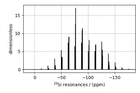
# The plot of the simulation before signal processing.
ax = plt.subplot(projection="csdm")
ax.plot(sim.methods[0].simulation.real, color="black", linewidth=1)
ax.invert_xaxis()
plt.tight_layout()
plt.show()

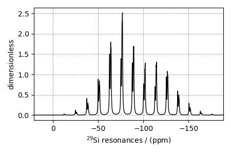
Step 6: Add post-simulation signal processing.

processor = sp.SignalProcessor(
    operations=[sp.IFFT(), apo.Exponential(FWHM="70 Hz"), sp.FFT()]
)
processed_data = processor.apply_operations(data=sim.methods[0].simulation)

# The plot of the simulation after signal processing.
ax = plt.subplot(projection="csdm")
ax.plot(processed_data.real, color="black", linewidth=1)
ax.invert_xaxis()
plt.tight_layout()
plt.show()

1

Hansen, M. R., Jakobsen, H. J., Skibsted, J., \(^{29}\text{Si}\) Chemical Shift Anisotropies in Calcium Silicates from High-Field \(^{29}\text{Si}\) MAS NMR Spectroscopy, Inorg. Chem. 2003, 42, 7, 2368-2377. DOI: 10.1021/ic020647f