Writing Custom methods (HahnEcho)

Writing custom methods using the Event objects.

import numpy as np
import matplotlib.pyplot as plt

from mrsimulator import Simulator, SpinSystem, Site, Coupling
from mrsimulator.method import Method, SpectralDimension, SpectralEvent, MixingEvent
from mrsimulator.spin_system.tensors import SymmetricTensor
from pprint import pprint

For demonstration, we will create two spin systems, one with a single site and other with two spin 1/2 sites.

S1 = Site(
    isotope="1H",
    isotropic_chemical_shift=10,  # in ppm
    shielding_symmetric=SymmetricTensor(zeta=-80, eta=0.25),  # zeta in ppm
)
S2 = Site(isotope="1H", isotropic_chemical_shift=-10)
S12 = Coupling(
    site_index=[0, 1], isotropic_j=100, dipolar=SymmetricTensor(D=2000, eta=0, alpha=0)
)

spin_system_1 = SpinSystem(sites=[S1], label="Uncoupled system")
spin_system_2 = SpinSystem(sites=[S1, S2], couplings=[S12], label="Coupled system")

Create a custom method

This example is a brief illustrate on how to write a custom method in mrsimulator. For in-depth description, please refer to the Method documentation.

In this example, we use two types of Event objects—SpectralEvent and MixingEvent to create a one-dimensional Hahn echo method.

hahn_echo = Method(
    channels=["1H"],
    magnetic_flux_density=9.4,  # in T
    rotor_angle=0,  # in rads
    rotor_frequency=0,  # in Hz
    spectral_dimensions=[
        SpectralDimension(
            count=512,
            spectral_width=2e4,  # in Hz
            events=[
                SpectralEvent(fraction=0.5, transition_queries=[{"ch1": {"P": [1]}}]),
                MixingEvent(query={"ch1": {"angle": np.pi, "phase": 0}}),
                SpectralEvent(fraction=0.5, transition_queries=[{"ch1": {"P": [-1]}}]),
            ],
        )
    ],
)

In the above code, we define the two SpectralEvent objects with fraction 0.5 and the transition_queries on channel-1 of P=[1] and P=[-1], respectively. Notice, the value for the P attribute is a list. Here, it is a list with a single integer. The list notation, [1], implies that the query selects all transitions where exactly one spin is undergoing a \(p=+1\) transition with the remaining spin at \(p=0\). A similar argument holds for [-1] query. By implementing query objects, we decouple the method from the spin system, i.e., once a method is defined, it can be used to simulate spectra from any given spin system. We will demonstrate this momentarily by simulating a Hahn echo spectrum from single and two-site spin systems.

Besides the SpectralEvent, you may also notice a MixingEvent sandwiched in-between the two SpectralEvent. A MixingEvent does not directly contribute to the frequencies. As the name suggests, a mixing event is used for the mixing of transitions in a multi-event method such as HahnEcho. In the above code, we define a mixing query on channel-1 by setting the attributes angle and phase to \(\pi\) and 0, respectively. There two parameters are analogous to the pulse angle and phase.

plt.figure(figsize=(4, 2))
hahn_echo.plot()
plt.show()

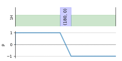
As mentioned before, a method object is decoupled from the spin system object. Notice, when we get the transition pathways from this method for a single-site spin system, we get a single transition pathway.

pprint(hahn_echo.get_transition_pathways(spin_system_1))

[|0.5⟩⟨-0.5| ⟶ |-0.5⟩⟨0.5|, weight=(1+0j)]

In the case of a homonuclear two-site spin 1/2 spin system, the same method returns four transition pathways.

pprint(hahn_echo.get_transition_pathways(spin_system_2))

[|-0.5, 0.5⟩⟨-0.5, -0.5| ⟶ |0.5, -0.5⟩⟨0.5, 0.5|, weight=(1+0j),
 |0.5, -0.5⟩⟨-0.5, -0.5| ⟶ |-0.5, 0.5⟩⟨0.5, 0.5|, weight=(1+0j),
 |0.5, 0.5⟩⟨-0.5, 0.5| ⟶ |-0.5, -0.5⟩⟨0.5, -0.5|, weight=(1+0j),
 |0.5, 0.5⟩⟨0.5, -0.5| ⟶ |-0.5, -0.5⟩⟨-0.5, 0.5|, weight=(1+0j)]

Create the Simulator object, add the method and spin system objects, and run the simulation.

sim = Simulator(spin_systems=[spin_system_1, spin_system_2], methods=[hahn_echo])
sim.config.decompose_spectrum = "spin_system"
sim.run()

The simulation from each spin system is stored as a dependent variable within the CSDM object. Use the split function to split the list of the dependent variables into a list of CSDM objects.

simulation_results = sim.methods[0].simulation.split()

# The plot of the two simulations.
fig, ax = plt.subplots(1, 2, figsize=(8.0, 3.0), subplot_kw={"projection": "csdm"})
for i in range(2):
    ax[i].plot(simulation_results[i].real, color="black", linewidth=1)
    ax[i].invert_xaxis()
plt.tight_layout()
plt.show()

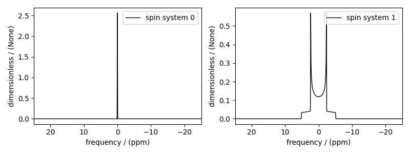
Notice, in the single-site spin system, the hahn echo refocuses the isotropic chemical shits and chemical shift anisotropies. The end result is a resonance at zero frequency. In the case of the two homonuclear spin 1/2 coupled spin system, the Hahn echo refocuses the isotropic chemical shits and chemical shift anisotropies, but not the dipolar and J couplings.