Amorphous material, ²⁹Si (I=1/2)

²⁹Si (I=1/2) simulation of amorphous material.

One of the advantages of the mrsimulator package is that it is a fast NMR spectrum simulation library. We can exploit this feature to simulate bulk spectra and eventually model amorphous materials. In this section, we illustrate how the mrsimulator library may be used in simulating the NMR spectrum of amorphous materials.

import numpy as np
import matplotlib.pyplot as plt
from scipy.stats import multivariate_normal

from mrsimulator import Simulator
from mrsimulator.method.lib import BlochDecaySpectrum
from mrsimulator.utils.collection import single_site_system_generator
from mrsimulator.method import SpectralDimension

Generating tensor parameter distribution

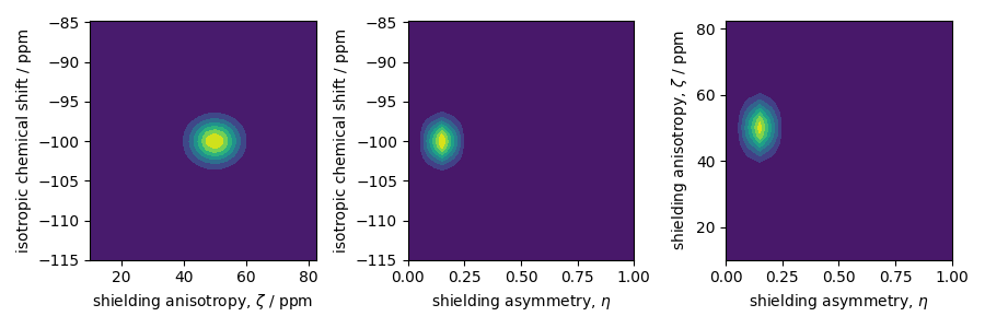
We model the amorphous material by assuming a distribution of interaction tensors. For example, a tri-variate normal distribution of the shielding tensor parameters, i.e., the isotropic chemical shift, the anisotropy parameter, \(\zeta\), and the asymmetry parameter, \(\eta\). In the following, we use pure NumPy and SciPy methods to generate the three-dimensional distribution, as follows,

mean = [-100, 50, 0.15]  # given as [isotropic chemical shift in ppm, zeta in ppm, eta].
covariance = [[3.25, 0, 0], [0, 26.2, 0], [0, 0, 0.002]]  # same order as the mean.

# range of coordinates along the three dimensions
iso_range = np.arange(100) * 0.3055 - 115  # in ppm
zeta_range = np.arange(30) * 2.5 + 10  # in ppm
eta_range = np.arange(21) / 20

# The coordinates grid
iso, zeta, eta = np.meshgrid(iso_range, zeta_range, eta_range, indexing="ij")
pos = np.asarray([iso, zeta, eta]).T

# Three-dimensional probability distribution function.
pdf = multivariate_normal(mean=mean, cov=covariance).pdf(pos).T

Here, iso, zeta, and eta are the isotropic chemical shift, nuclear shielding anisotropy, and nuclear shielding asymmetry coordinates of the 3D-grid system over which the multivariate normal probability distribution is evaluated. The mean of the distribution is given by the variable mean and holds a value of -100 ppm, 50 ppm, and 0.15 for the isotropic chemical shift, nuclear shielding anisotropy, and nuclear shielding asymmetry parameter, respectively. Similarly, the variable covariance holds the covariance matrix of the multivariate normal distribution. The two-dimensional projections from this three-dimensional distribution are shown below.

_, ax = plt.subplots(1, 3, figsize=(9, 3))

# isotropic shift v.s. shielding anisotropy
ax[0].contourf(zeta_range, iso_range, pdf.sum(axis=2))
ax[0].set_xlabel(r"shielding anisotropy, $\zeta$ / ppm")
ax[0].set_ylabel("isotropic chemical shift / ppm")

# isotropic shift v.s. shielding asymmetry
ax[1].contourf(eta_range, iso_range, pdf.sum(axis=1))
ax[1].set_xlabel(r"shielding asymmetry, $\eta$")
ax[1].set_ylabel("isotropic chemical shift / ppm")

# shielding anisotropy v.s. shielding asymmetry
ax[2].contourf(eta_range, zeta_range, pdf.sum(axis=0))
ax[2].set_xlabel(r"shielding asymmetry, $\eta$")
ax[2].set_ylabel(r"shielding anisotropy, $\zeta$ / ppm")

plt.tight_layout()
plt.show()

Create the Simulator object

Spin system:

Let’s create the sites and single-site spin system objects from these parameters. Use the single_site_system_generator() utility function to generate single-site spin systems. # Here, iso, zeta, and eta are the array of tensor parameter coordinates, and pdf is the array of the corresponding amplitudes.

spin_systems = single_site_system_generator(
    isotope="29Si",
    isotropic_chemical_shift=iso,
    shielding_symmetric={"zeta": zeta, "eta": eta},
    abundance=pdf,
)

Method:

Let’s also create a Bloch decay spectrum method.

method = BlochDecaySpectrum(
    channels=["29Si"],
    rotor_frequency=0,  # in Hz
    rotor_angle=0,  # in rads
    spectral_dimensions=[
        SpectralDimension(spectral_width=25000, reference_offset=-7000)  # values in Hz
    ],
)

The above method simulates a static \(^{29}\text{Si}\) spectrum at 9.4 T field (default value).

Simulator:

Now that we have the spin systems and the method, create the simulator object and add the respective objects.

sim = Simulator(spin_systems=spin_systems, methods=[method])

Static spectrum

Observe the static \(^{29}\text{Si}\) NMR spectrum simulation.

sim.run()

The plot of the simulation.

plt.figure(figsize=(4.25, 3.0))
ax = plt.subplot(projection="csdm")
ax.plot(sim.methods[0].simulation.real, color="black", linewidth=1)
ax.invert_xaxis()
plt.tight_layout()
plt.show()

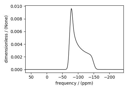
Note

The broad spectrum seen in the above figure is a result of spectral averaging of spectra arising from a distribution of shielding tensors. There is no line-broadening filter applied to the spectrum.

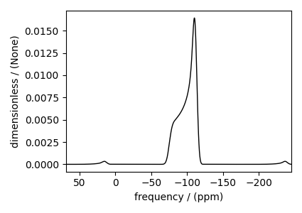
Spinning sideband simulation at \(90^\circ\)

Here is an example of a sideband simulation, spinning at a 90-degree angle.

sim.methods[0] = BlochDecaySpectrum(
    channels=["29Si"],
    rotor_frequency=5000,  # in Hz
    rotor_angle=1.57079,  # in rads, equivalent to 90 deg.
    spectral_dimensions=[
        SpectralDimension(spectral_width=25000, reference_offset=-7000)  # values in Hz
    ],
)
sim.config.number_of_sidebands = 8  # eight sidebands are sufficient for this example
sim.run()

The plot of the simulation.

plt.figure(figsize=(4.25, 3.0))
ax = plt.subplot(projection="csdm")
ax.plot(sim.methods[0].simulation.real, color="black", linewidth=1)
ax.invert_xaxis()
plt.tight_layout()
plt.show()

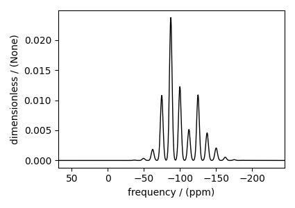
Spinning sideband simulation at the magic angle

Here is another example of a sideband simulation at the magic angle.

sim.methods[0] = BlochDecaySpectrum(
    channels=["29Si"],
    rotor_frequency=1000,  # in Hz
    rotor_angle=54.7356 * np.pi / 180.0,  # in rads
    spectral_dimensions=[
        SpectralDimension(spectral_width=25000, reference_offset=-7000)  # values in Hz
    ],
)
sim.config.number_of_sidebands = 16  # sixteen sidebands are sufficient for this example
sim.run()

The plot of the simulation.

plt.figure(figsize=(4.25, 3.0))
ax = plt.subplot(projection="csdm")
ax.plot(sim.methods[0].simulation.real, color="black", linewidth=1)
ax.invert_xaxis()
plt.tight_layout()
plt.show()