Rb₂CrO₄, ⁸⁷Rb (I=3/2) COASTER¶

⁸⁷Rb (I=3/2) Correlation of anisotropies separated through echo refocusing (COASTER) simulation.

The following is a Correlation of Anisotropies Separated Through Echo Refocusing (COASTER) simulation of \(\text{Rb}_2\text{CrO}_4\). The Rb site with the smaller quadrupolar interaction is selectively observed and reported by Ash et al. [1]. The following is the simulation based on the published tensor parameters.

import numpy as np
import matplotlib.pyplot as plt

from mrsimulator import Simulator, SpinSystem, Site
from mrsimulator import signal_processor as sp
from mrsimulator.spin_system.tensors import SymmetricTensor
from mrsimulator.method import Method, SpectralDimension, SpectralEvent, MixingEvent

Generate the site and spin system objects.

site = Site(
    isotope="87Rb",
    isotropic_chemical_shift=-9,  # in ppm
    shielding_symmetric=SymmetricTensor(zeta=110, eta=0),
    quadrupolar=SymmetricTensor(
        Cq=3.5e6,  # in Hz
        eta=0.36,
        alpha=0,  # in rads
        beta=70 * 3.14159 / 180,  # in rads
        gamma=0,  # in rads
    ),
)
spin_system = SpinSystem(sites=[site])

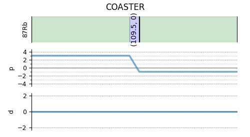
Use the generic Method class to simulate a 2D COASTER spectrum by customizing the method parameters, as shown below.

By default, all transitions selected from a SpectralEvent connect to all selected transitions from the following SpectralEvent if no MixingEvent is defined between them. Here, we define a MixingEvent with an angle of 109.5 degrees to connect the 3Q to 1Q transitions.

coaster = Method(
    name="COASTER",
    channels=["87Rb"],
    magnetic_flux_density=9.4,  # in T
    rotor_angle=70.12 * np.pi / 180,  # in rads
    rotor_frequency=np.inf,
    spectral_dimensions=[
        SpectralDimension(
            count=512,
            spectral_width=4e4,  # in Hz
            reference_offset=-8e3,  # in Hz
            label="$\\omega_1$ (CSA)",
            events=[
                SpectralEvent(transition_queries=[{"ch1": {"P": [3], "D": [0]}}]),
                MixingEvent(query={"ch1": {"angle": np.pi * 109.5 / 180, "phase": 0}}),
            ],
        ),
        # The last spectral dimension block is the direct-dimension
        SpectralDimension(
            count=512,
            spectral_width=8e3,  # in Hz
            reference_offset=-4e3,  # in Hz
            label="$\\omega_2$ (Q)",
            events=[SpectralEvent(transition_queries=[{"ch1": {"P": [-1], "D": [0]}}])],
        ),
    ],
    affine_matrix=[[1, 0], [1 / 4, 3 / 4]],
)

# A graphical representation of the method object.
plt.figure(figsize=(5, 2.75))
coaster.plot()
plt.show()

Create the Simulator object, add the method and spin system objects, and run the simulation.

sim = Simulator(spin_systems=[spin_system], methods=[coaster])

# configure the simulator object. For non-coincidental tensors, set the value of the
# `integration_volume` attribute to `hemisphere`.
sim.config.integration_volume = "hemisphere"
sim.run()

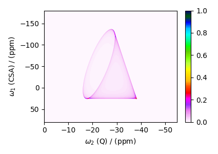
The plot of the simulation.

dataset = sim.methods[0].simulation

plt.figure(figsize=(4.25, 3.0))
ax = plt.subplot(projection="csdm")
cb = ax.imshow(dataset.real / dataset.real.max(), aspect="auto", cmap="gist_ncar_r")
plt.colorbar(cb)
ax.set_xlim(-0, -55)
ax.set_ylim(80, -180)
plt.tight_layout()
plt.show()

Add post-simulation signal processing.

processor = sp.SignalProcessor(
    operations=[
        # Gaussian convolution along both dimensions.
        sp.IFFT(dim_index=(0, 1)),
        sp.apodization.Gaussian(FWHM="0.15 kHz", dim_index=0),
        sp.apodization.Gaussian(FWHM="0.15 kHz", dim_index=1),
        sp.FFT(dim_index=(0, 1)),
    ]
)
processed_dataset = processor.apply_operations(dataset=dataset)
processed_dataset /= processed_dataset.max()

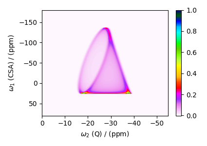
The plot of the simulation after signal processing.

plt.figure(figsize=(4.25, 3.0))
ax = plt.subplot(projection="csdm")
cb = ax.imshow(processed_dataset.real, cmap="gist_ncar_r", aspect="auto")
plt.colorbar(cb)
ax.set_xlim(-0, -55)
ax.set_ylim(80, -180)
plt.tight_layout()
plt.show()

Total running time of the script: (0 minutes 1.157 seconds)

Gallery generated by Sphinx-Gallery