Note
Go to the end to download the full example code.
³¹P MAS NMR of crystalline Na2PO4 (CSA)
In this example, we illustrate the use of the mrsimulator objects to
create a CSA fitting model using Simulator and SignalProcessor objects,
use the fitting model to perform a least-squares analysis, and
extract the fitting parameters from the model.
We use the LMFIT library to fit the spectrum. The following example shows the least-squares fitting procedure applied to the \(^{31}\text{P}\) MAS NMR spectrum of \(\text{Na}_{2}\text{PO}_{4}\). The following experimental dataset is a part of DMFIT [1] examples. We thank Dr. Dominique Massiot for sharing the dataset.
Start by importing the relevant modules.
import csdmpy as cp
import numpy as np
import matplotlib.pyplot as plt
from lmfit import Minimizer

from mrsimulator import Simulator, SpinSystem, Site
from mrsimulator.method.lib import BlochDecaySpectrum
from mrsimulator import signal_processor as sp
from mrsimulator.utils import spectral_fitting as sf
from mrsimulator.utils import get_spectral_dimensions
from mrsimulator.spin_system.tensors import SymmetricTensor
Import the dataset
Import the experimental data. We use dataset file serialized with the CSDM file-format, using the csdmpy module.
host = "https://nmr.cemhti.cnrs-orleans.fr/Dmfit/Help/csdm/"
filename = "31P Phosphate 6kHz.csdf"
experiment = cp.load(host + filename)
# For spectral fitting, we only focus on the real part of the complex dataset
experiment = experiment.real
# Convert the dimension coordinates from Hz to ppm.
experiment.x[0].to("ppm", "nmr_frequency_ratio")
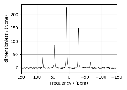
# plot of the dataset.
plt.figure(figsize=(4.25, 3.0))
ax = plt.subplot(projection="csdm")
ax.plot(experiment, color="black", linewidth=0.5, label="Experiment")
ax.set_xlim(150, -150)
plt.grid()
plt.tight_layout()
plt.show()
Estimate noise statistics from the dataset
coords = experiment.dimensions[0].coordinates
noise_region = np.where(coords < -100e-6)
noise_data = experiment[noise_region]

plt.figure(figsize=(3.75, 2.5))
ax = plt.subplot(projection="csdm")
ax.plot(noise_data, label="noise")
plt.title("Noise section")
plt.axis("off")
plt.tight_layout()
plt.show()

noise_mean, sigma = experiment[noise_region].mean(), experiment[noise_region].std()
noise_mean, sigma
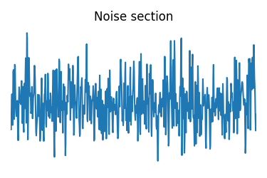
(<Quantity -1.6514109>, <Quantity 1.5352644>)
Create a fitting model
A fitting model is a composite of Simulator and SignalProcessor objects.
Step 1: Create initial guess sites and spin systems
P_31 = Site(
    isotope="31P",
    isotropic_chemical_shift=5.0,  # in ppm,
    shielding_symmetric=SymmetricTensor(zeta=-80, eta=0.5),  # zeta in Hz
)

spin_systems = [SpinSystem(sites=[P_31])]
Step 2: Create the method object. Create an appropriate method object that closely resembles the technique used in acquiring the experimental dataset. The attribute values of this method must meet the experimental conditions, including the acquisition channels, the magnetic flux density, rotor angle, rotor frequency, and the spectral/spectroscopic dimension.
In the following example, we set up a Bloch decay spectrum method where the
spectral/spectroscopic dimension information, i.e., count, spectral_width, and the
reference_offset, is extracted from the CSDM dimension metadata using the
get_spectral_dimensions() utility function. The remaining
attribute values are set to the experimental conditions.
# get the count, spectral_width, and reference_offset information from the experiment.
spectral_dims = get_spectral_dimensions(experiment)

MAS = BlochDecaySpectrum(
    channels=["31P"],
    magnetic_flux_density=9.395,  # in T
    rotor_frequency=6000,  # in Hz
    spectral_dimensions=spectral_dims,
    experiment=experiment,  # experimental dataset
)
Step 3: Create the Simulator object and add the method and spin system objects.
Step 4: Create a SignalProcessor class object and apply the post-simulation signal processing operations.
processor = sp.SignalProcessor(
    operations=[
        sp.IFFT(),
        sp.apodization.Exponential(FWHM="0.3 kHz"),
        sp.FFT(),
        sp.Scale(factor=3000),
        sp.baseline.ConstantOffset(offset=-2),
    ]
)
processed_dataset = processor.apply_operations(dataset=sim.methods[0].simulation).real
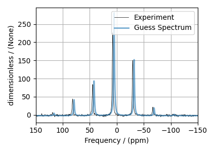
Step 5: The plot of the dataset and the guess spectrum.
plt.figure(figsize=(4.25, 3.0))
ax = plt.subplot(projection="csdm")
ax.plot(experiment, color="black", linewidth=0.5, label="Experiment")
ax.plot(processed_dataset, linewidth=2, alpha=0.6, label="Guess Spectrum")
ax.set_xlim(150, -150)
plt.legend()
plt.grid()
plt.tight_layout()
plt.show()
Least-squares minimization with LMFIT
Once you have a fitting model, you need to create the list of parameters to use in the
least-squares minimization. For this, you may use the
Parameters class from LMFIT,
as described in the previous example.
Here, we make use of a utility function,
make_LMFIT_params(), to simplifies the
LMFIT parameters generation process. By default, the function only creates parameters
from the SpinSystem and SignalProcessor objects. Often, in spectrum with sidebands,
spinning speed may not be accurately known; and is, therefore, included as a fitting
parameter. To include a keyword from the method object, use the include argument
of the function, as follows,
Step 6: Create a list of parameters.
params = sf.make_LMFIT_params(sim, processor, include={"rotor_frequency"})
The make_LMFIT_params parses the instances of the Simulator and the
PostSimulator objects for parameters and returns a LMFIT Parameters object.
Customize the Parameters:
You may customize the parameters list, params, as desired. Here, we remove the
abundance parameter.
params.pop("sys_0_abundance")
print(params.pretty_print(columns=["value", "min", "max", "vary", "expr"]))
Name                                       Value      Min      Max     Vary     Expr
SP_0_operation_1_Exponential_FWHM            0.3     -inf      inf     True     None
SP_0_operation_3_Scale_factor               3000     -inf      inf     True     None
SP_0_operation_4_ConstantOffset_offset        -2     -inf      inf     True     None
mth_0_rotor_frequency                       6000     5900     6100     True     None
sys_0_site_0_isotropic_chemical_shift          5     -inf      inf     True     None
sys_0_site_0_shielding_symmetric_eta         0.5        0        1     True     None
sys_0_site_0_shielding_symmetric_zeta        -80     -inf      inf     True     None
None
Step 7: Perform the least-squares minimization.
A method object queries every spin system for a list of transition pathways that are
relevant to the given method. Since the method and the number of spin systems remains
unchanged during the least-squares analysis, a one-time query is sufficient. To avoid
querying for the transition pathways at every iteration in a least-squares fitting,
call the optimize() method to pre-compute the
pathways.
For the user’s convenience, we
also provide a utility function,
LMFIT_min_function(), for evaluating the
difference vector between the simulation and experiment, based on
the parameters update. You may use this function directly to instantiate the
LMFIT Minimizer class where fcn_args and fcn_kws are arguments passed to the
function, as follows,
opt = sim.optimize()  # Pre-compute transition pathways
minner = Minimizer(
    sf.LMFIT_min_function,
    params,
    fcn_args=(sim, processor, sigma),
    fcn_kws={"opt": opt},
)
result = minner.minimize()
result
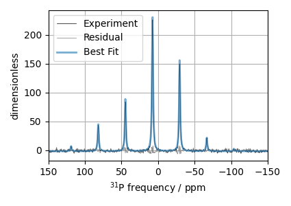
Step 8: The plot of the fit, measurement, and residuals.
# Best fit spectrum
best_fit = sf.bestfit(sim, processor)[0].real
residuals = sf.residuals(sim, processor)[0].real

plt.figure(figsize=(4.25, 3.0))
ax = plt.subplot(projection="csdm")
ax.plot(experiment, color="black", linewidth=0.5, label="Experiment")
ax.plot(residuals, color="gray", linewidth=0.5, label="Residual")
ax.plot(best_fit, linewidth=2, alpha=0.6, label="Best Fit")
ax.set_xlabel(r"$^{31}$P frequency / ppm")
ax.set_xlim(150, -150)
plt.legend()
plt.grid()
plt.tight_layout()
plt.show()
Total running time of the script: (0 minutes 2.218 seconds)