Gaussian Apodization

In this example, we will use the Gaussian class to perform a Gaussian convolution on an example dataset. The function used for this apodization is defined as follows

(45)\[f(x) = e^{-2 \pi^2 \sigma^2 x^2}\]

where \(\sigma\) is the standard deviation of the Gaussian function and is parameterized by the full width as half maximum (FWHM) as

(46)\[\sigma = \frac{\text{FWHM}}{2\sqrt{2\ln 2}}\]

Below we import the necessary modules sphinx_gallery_thumbnail_number = 1

import csdmpy as cp
import numpy as np
from mrsimulator import signal_processor as sp

First we create processor, an instance of the SignalProcessor class. The required attribute of the SignalProcessor class, operations, is a list of operations to which we add a Gaussian object sandwiched between two Fourier transformations.

processor = sp.SignalProcessor(
    operations=[
        sp.IFFT(),
        sp.apodization.Gaussian(FWHM="75 Hz"),
        sp.FFT(),
    ]
)

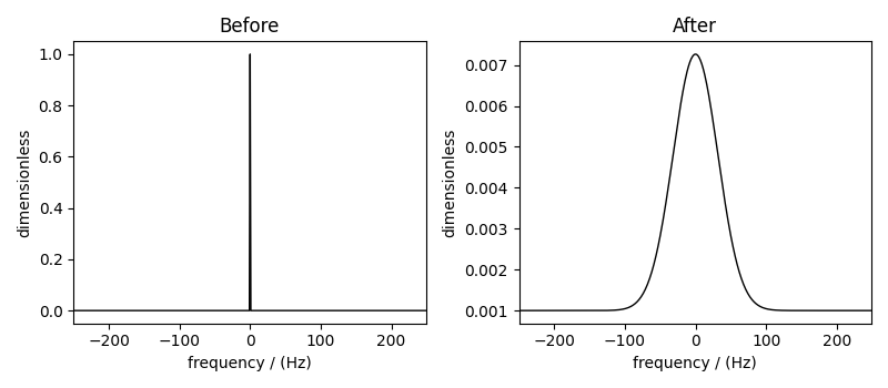
Next we create a CSDM object with a test dataset which our signal processor will operate on. Here, the dataset spans 500 Hz with a delta function centered at 0 Hz.

test_data = np.zeros(500)
test_data[250] = 1
csdm_object = cp.CSDM(
    dependent_variables=[cp.as_dependent_variable(test_data)],
    dimensions=[cp.LinearDimension(count=500, increment="1 Hz", complex_fft=True)],
)

Now to apply the processor to the CSDM object, use the apply_operations() method as follows

processed_dataset = processor.apply_operations(dataset=csdm_object).real

To see the results of the Gaussian apodization, we create a simple plot using the matplotlib library.

import matplotlib.pyplot as plt

fig, ax = plt.subplots(1, 2, figsize=(8, 3.5), subplot_kw={"projection": "csdm"})
ax[0].plot(csdm_object, color="black", linewidth=1)
ax[0].set_title("Before")
ax[1].plot(processed_dataset.real, color="black", linewidth=1)
ax[1].set_title("After")
plt.tight_layout()
plt.show()