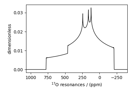
Non-coincidental Quad and CSA, ¹⁷O (I=5/2)¶

¹⁷O (I=5/2) quadrupolar static spectrum simulation.

The following example illustrates the simulation of NMR spectra arising from non-coincidental quadrupolar and shielding tensors. The tensor parameter values for the simulation are obtained from Yamada et al. [1], for the \(^{17}\text{O}\) site in benzanilide.

Warning

The Euler angles representation used by Yamada et al is different from the representation used in mrsimulator. The resulting simulation might not resemble the published spectrum.

import numpy as np
import matplotlib.pyplot as plt

from mrsimulator import Simulator, SpinSystem, Site
from mrsimulator.method.lib import BlochDecayCTSpectrum
from mrsimulator.spin_system.tensors import SymmetricTensor
from mrsimulator.method import SpectralDimension

Step 1: Create the spin system.

site = Site(
    isotope="17O",
    isotropic_chemical_shift=320,  # in ppm
    shielding_symmetric=SymmetricTensor(zeta=376.667, eta=0.345),
    quadrupolar=SymmetricTensor(
        Cq=8.97e6,  # in Hz
        eta=0.15,
        alpha=5 * np.pi / 180,
        beta=np.pi / 2,
        gamma=70 * np.pi / 180,
    ),
)
spin_system = SpinSystem(sites=[site])

Step 2: Create a central transition selective Bloch decay spectrum method.

method = BlochDecayCTSpectrum(
    channels=["17O"],
    magnetic_flux_density=11.74,  # in T
    rotor_frequency=0,  # in Hz
    spectral_dimensions=[
        SpectralDimension(
            count=1024,
            spectral_width=1e5,  # in Hz
            reference_offset=22500,  # in Hz
            label=r"$^{17}$O resonances",
        )
    ],
)

Step 3: Create the Simulator object and add method and spin system objects.

sim = Simulator()
sim.spin_systems = [spin_system]  # add the spin system
sim.methods = [method]  # add the method

# Since the spin system have non-zero Euler angles, set the integration_volume to
# hemisphere.
sim.config.integration_volume = "hemisphere"

Step 4: Simulate the spectrum.

sim.run()

# The plot of the simulation before signal processing.
plt.figure(figsize=(4.25, 3.0))
ax = plt.subplot(projection="csdm")
ax.plot(sim.methods[0].simulation.real, color="black", linewidth=1)
ax.invert_xaxis()
plt.tight_layout()
plt.show()

Total running time of the script: ( 0 minutes 0.242 seconds)

Gallery generated by Sphinx-Gallery