Coupled spin-1/2 (CSA + heteronuclear dipolar + J-couplings)

¹³C-¹H sideband simulation

The following simulation is an example by Edén [1] from Computer Simulations in Solid-State NMR.III.Powder Averaging. The simulation consists of sideband spectra from a 13C-1H coupled spin system computed at various spinning frequencies with different relative tensor orientations between the nuclear shielding and dipolar interaction tensors.

import numpy as np
import matplotlib.pyplot as plt

from mrsimulator import Simulator, SpinSystem, Site, Coupling
from mrsimulator.method.lib import BlochDecaySpectrum
from mrsimulator import signal_processor as sp
from mrsimulator.spin_system.tensors import SymmetricTensor
from mrsimulator.method import SpectralDimension

Spin Systems

Here, we create three 13C-1H spin systems with different relative orientations between the shielding and dipolar tensors. The Euler angle orientations \(\alpha=\gamma=0\) and \(\beta\) values are listed below.

beta_orientation = [np.pi / 6, 5 * np.pi / 18, np.pi / 2]

# The `variable` spin_systems is a list of three coupled 13C-1H spin systems with
# different relative shielding and dipolar tensor orientation.
spin_systems = [
    SpinSystem(
        sites=[
            Site(
                isotope="13C",
                isotropic_chemical_shift=0.0,  # in ppm
                shielding_symmetric=SymmetricTensor(
                    zeta=18.87562,  # in ppm
                    eta=0.4,
                    beta=beta,
                ),
            ),
            Site(
                isotope="1H",
                isotropic_chemical_shift=0.0,  # in ppm
            ),
        ],
        couplings=[
            Coupling(
                site_index=[0, 1], isotropic_j=200.0, dipolar=SymmetricTensor(D=-2.1e4)
            )
        ],
    )
    for beta in beta_orientation
]

Methods

Next, we create methods to simulate the sideband manifolds for the above spin systems at four spinning rates: 3 kHz, 5 kHz, 8 kHz, 12 kHz.

spin_rates = [3e3, 5e3, 8e3, 12e3]  # in Hz

# The variable `methods` is a list of four BlochDecaySpectrum methods.
methods = [
    BlochDecaySpectrum(
        channels=["13C"],
        magnetic_flux_density=9.4,  # in T
        rotor_frequency=vr,  # in Hz
        spectral_dimensions=[SpectralDimension(count=2048, spectral_width=8.0e4)],
    )
    for vr in spin_rates
]

Simulator

Create the Simulator object and add the method and the spin system objects.

sim = Simulator()
sim.spin_systems = spin_systems  # add the three spin systems
sim.methods = methods  # add the four methods
sim.config.integration_volume = "hemisphere"  # set averaging to hemisphere
# config to decompose spectrum to individual spin systems.
sim.config.decompose_spectrum = "spin_system"

The run command will simulate twelve spectra corresponding to the three spin systems evaluated at four different methods (spinning speeds).

sim.run()

Post-Simulation Processing

Add post-simulation signal processing.

processor = sp.SignalProcessor(
    operations=[
        sp.IFFT(),
        sp.apodization.Exponential(FWHM="50 Hz"),
        sp.FFT(),
    ]
)
# apply the same post-simulation processing to all the twelve simulations.
processed_dataset = [
    processor.apply_operations(dataset=method.simulation) for method in sim.methods
]

Plot

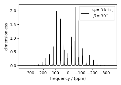
Let’s first plot a single simulation, the one corresponding to a relative orientation of \(\beta=30^\circ\) between the shielding and dipolar tensors and a spinning speed of 3 kHz.

plt.figure(figsize=(4.25, 3.0))
ax = plt.subplot(projection="csdm")
ax.plot(
    processed_dataset[0].split()[0].real,
    color="black",
    linewidth=1,
    label="$\\nu_r=$3 kHz, \n $\\beta=30^\\circ$",
)
ax.legend()
ax.invert_xaxis()
plt.tight_layout()
plt.show()

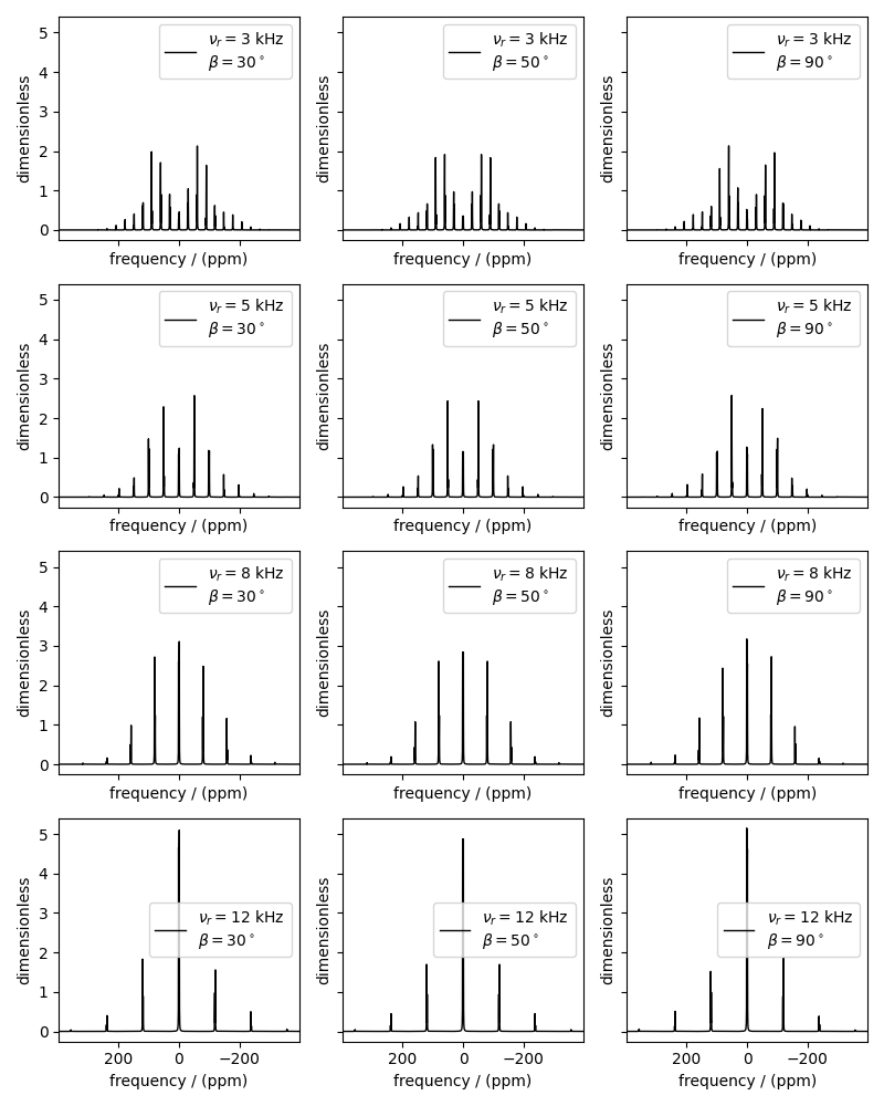
The following is a grid plot showing all twelve simulations. For reference, see Figure 11 from [1].

fig, ax = plt.subplots(
    nrows=4,
    ncols=3,
    subplot_kw={"projection": "csdm"},
    sharex=True,
    sharey=True,
    figsize=(8, 10.0),
)
for i, datum in enumerate(processed_dataset):
    datum_spin_sys = datum.split()  # get simulation from the three spin systems.
    for j, item in enumerate(datum_spin_sys):
        ax[i, j].plot(
            item.real,
            color="black",
            linewidth=1,
            label=(
                f"$\\nu_r={spin_rates[i]/1e3: .0f}$ kHz \n"
                f"$\\beta={beta_orientation[j]/np.pi*180: .0f}^\\circ$"
            ),
        )
        ax[i, j].invert_xaxis()
        ax[i, j].legend()
plt.tight_layout()
plt.show()

[1] (1,2)

Edén, M. Computer Simulations in Solid-State NMR. III. Powder Averaging, Concepts in Magnetic Resonance Part A, Vol. 18A(1) 24–55 (2003). DOI: doi.org/10.1002/cmr.a.10065