Note
Go to the end to download the full example code.
Amorphous material, ²⁷Al (I=5/2)
²⁷Al (I=5/2) simulation of amorphous material.
import numpy as np
import matplotlib.pyplot as plt
from scipy.stats import multivariate_normal

from mrsimulator import Simulator
from mrsimulator.method.lib import BlochDecayCTSpectrum
from mrsimulator.utils.collection import single_site_system_generator
from mrsimulator.method import SpectralDimension
In this section, we illustrate the simulation of a quadrupolar spectrum arising from a distribution of the electric field gradient (EFG) tensors from an amorphous material. We proceed by assuming a multi-variate normal distribution, as follows,
mean = [20, 6.5, 0.3]  # given as [isotropic chemical shift in ppm, Cq in MHz, eta].
covariance = [[1.98, 0, 0], [0, 4.9, 0], [0, 0, 0.0016]]  # same order as the mean.

# range of coordinates along the three dimensions
iso_range = np.arange(40)  # in ppm
Cq_range = np.arange(80) / 3 - 5  # in MHz
eta_range = np.arange(21) / 20

# The coordinates grid
iso, Cq, eta = np.meshgrid(iso_range, Cq_range, eta_range, indexing="ij")
pos = np.asarray([iso, Cq, eta]).T

# Three-dimensional probability distribution function.
pdf = multivariate_normal(mean=mean, cov=covariance).pdf(pos).T
Here, iso, Cq, and eta are the isotropic chemical shift, the quadrupolar
coupling constant, and quadrupolar asymmetry coordinates of the 3D-grid
system over which the multivariate normal probability distribution is evaluated. The
mean of the distribution is given by the variable mean and holds a value of 20
ppm, 6.5 MHz, and 0.3 for the isotropic chemical shift, the quadrupolar coupling
constant, and quadrupolar asymmetry parameter, respectively. Similarly, the variable
covariance holds the covariance matrix of the multivariate normal distribution.
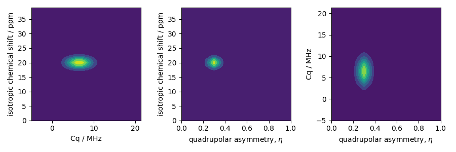
The two-dimensional projections from this three-dimensional distribution are shown
below.
_, ax = plt.subplots(1, 3, figsize=(9, 3))

# isotropic shift v.s. quadrupolar coupling constant
ax[0].contourf(Cq_range, iso_range, pdf.sum(axis=2))
ax[0].set_xlabel("Cq / MHz")
ax[0].set_ylabel("isotropic chemical shift / ppm")

# isotropic shift v.s. quadrupolar asymmetry
ax[1].contourf(eta_range, iso_range, pdf.sum(axis=1))
ax[1].set_xlabel(r"quadrupolar asymmetry, $\eta$")
ax[1].set_ylabel("isotropic chemical shift / ppm")

# quadrupolar coupling constant v.s. quadrupolar asymmetry
ax[2].contourf(eta_range, Cq_range, pdf.sum(axis=0))
ax[2].set_xlabel(r"quadrupolar asymmetry, $\eta$")
ax[2].set_ylabel("Cq / MHz")

plt.tight_layout()
plt.show()
Let’s create the site and spin system objects from these parameters. Note, we create
single-site spin systems for optimum performance.
Use the single_site_system_generator() utility
function to generate single-site spin systems.
spin_systems = single_site_system_generator(
    isotope="27Al",
    isotropic_chemical_shift=iso,
    quadrupolar={"Cq": Cq * 1e6, "eta": eta},  # Cq in Hz
    abundance=pdf,
)
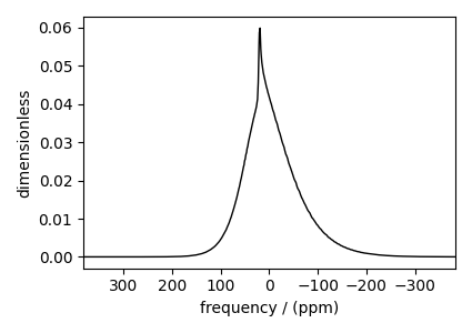
Static spectrum
Observe the static \(^{27}\text{Al}\) NMR spectrum simulation. First, create a central transition selective Bloch decay spectrum method.
static_method = BlochDecayCTSpectrum(
    channels=["27Al"],
    rotor_frequency=0,  # in Hz
    rotor_angle=0,  # in rads
    spectral_dimensions=[SpectralDimension(spectral_width=80000)],
)
Create the simulator object and add the spin systems and method.
sim = Simulator(spin_systems=spin_systems, methods=[static_method])
sim.run()
The plot of the corresponding spectrum.
plt.figure(figsize=(4.25, 3.0))
ax = plt.subplot(projection="csdm")
ax.plot(sim.methods[0].simulation.real, color="black", linewidth=1)
ax.invert_xaxis()
plt.tight_layout()
plt.show()
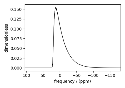
Spinning sideband simulation at the magic angle
Simulation of the same spin systems at the magic angle and spinning at 25 kHz.
MAS_method = BlochDecayCTSpectrum(
    channels=["27Al"],
    rotor_frequency=25000,  # in Hz
    rotor_angle=54.735 * np.pi / 180.0,  # in rads
    spectral_dimensions=[
        SpectralDimension(spectral_width=30000, reference_offset=-4000)  # values in Hz
    ],
)
sim.methods[0] = MAS_method
Configure the sim object to calculate up to 4 sidebands, and run the simulation.
and the corresponding plot.
plt.figure(figsize=(4.25, 3.0))
ax = plt.subplot(projection="csdm")
ax.plot(sim.methods[0].simulation.real, color="black", linewidth=1)
ax.invert_xaxis()
plt.tight_layout()
plt.show()
Total running time of the script: (0 minutes 13.276 seconds)