¹H COSY

A simple example of the phase-sensitive COSY experiment with two coupled ¹H nuclei.

import numpy as np
from mrsimulator import Simulator
from mrsimulator.method.query import Rotation
from mrsimulator import Method, SpectralDimension
from mrsimulator.method import SpectralEvent, RotationEvent
from mrsimulator.spin_system.isotope import Isotope
from mrsimulator import Site, Coupling, SpinSystem
from mrsimulator import signal_processor as sp

import matplotlib.pyplot as plt

Generate the site, coupling, and spin system objects.

site_A = Site(isotropic_chemical_shift=2.0)
site_X = Site(isotropic_chemical_shift=3.0)

coupling_AX = Coupling(site_index=[0, 1], isotropic_j=20)

ax_system = SpinSystem(sites=[site_A, site_X], couplings=[coupling_AX])

Create methods for the path and antipath of the COSY experiment

p_plus_query = [{"ch1": {"P": [+1]}}]
p_minus_query = [{"ch1": {"P": [-1]}}]
trans_queries = [
    p_minus_query,
    p_plus_query,
]

# Simulate a H-1 spectrum at 300 MHz |\label{ln:H1}|
H1 = Isotope(symbol="1H")
H1_ref_freq = 300  # MHz
B0 = H1.ref_freq_to_B0(H1_ref_freq * 1e6)  #
# Set the spectral width and reference offset |\label{ln:H1sw}|
sw = 1.5 * H1_ref_freq
offset = 2.5 * H1_ref_freq
offset_sign = [1, -1]

methods = [
    Method(
        channels=["1H"],
        magnetic_flux_density=B0,
        spectral_dimensions=[
            SpectralDimension(
                count=2048,
                spectral_width=sw,  # in Hz
                reference_offset=o_sgn * offset,  # in Hz
                events=[
                    SpectralEvent(transition_queries=t_queries),
                    RotationEvent(ch1=Rotation(angle=np.pi / 2, phase=-np.pi / 2)),
                ],
            ),
            SpectralDimension(
                count=2048,
                spectral_width=sw,  # in Hz
                reference_offset=offset,  # in Hz
                events=[SpectralEvent(transition_queries=[{"ch1": {"P": [-1]}}])],
            ),
        ],
    )
    for o_sgn, t_queries in zip(offset_sign, trans_queries)
]

Create the Simulator object with the spin system and two methods, and run the simulation.

sim = Simulator(spin_systems=[ax_system], methods=methods)
sim.config.integration_density = 1
sim.config.number_of_sidebands = 1
sim.run()

Build the processor, and apply the broadening and tophat apodization to all datasets. Perform hypercomplex processing by flipping the antipath and adding it to the path signal.

proc = sp.SignalProcessor(
    operations=[
        sp.IFFT(dim_index=(0, 1)),
        sp.apodization.TopHat(rising_edge="0 s", dim_index=0),
        sp.apodization.TopHat(rising_edge="0 s", dim_index=1),
        sp.apodization.Exponential(FWHM="1 Hz", dim_index=0),
        sp.apodization.Exponential(FWHM="1 Hz", dim_index=1),
        sp.FFT(dim_index=(0, 1)),
    ]
)

processed_path = proc.apply_operations(dataset=sim.methods[0].simulation)
processed_antipath = proc.apply_operations(dataset=sim.methods[1].simulation)

flipped = processed_antipath.fft(axis=0).conj().fft(axis=0)
flipped.dimensions[1] = processed_path.dimensions[1]

phase_sensitive_COSY = flipped + processed_path

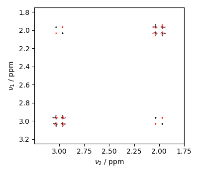
Plot the spectrum

max_amp = phase_sensitive_COSY.real.max()
levels = np.linspace(-max_amp, max_amp, 30)  # levels from -max_amp to max_amp
options = dict(alpha=0.75, linewidths=0.5)  # plot options

# Separate positive and negative levels
positive_levels = levels[levels > 0]
negative_levels = levels[levels < 0]

# Create a figure
fig, ax = plt.subplots(1, 1, figsize=(4, 3.5), subplot_kw={"projection": "csdm"})
ax.contour(phase_sensitive_COSY.real, levels=positive_levels, colors="k", **options)
ax.contour(phase_sensitive_COSY.real, levels=negative_levels, colors="r", **options)
ax.invert_xaxis()
ax.invert_yaxis()
ax.set_ylabel("$\\nu_1$ / ppm")
ax.set_xlabel("$\\nu_2$ / ppm")

plt.tight_layout()
plt.show()

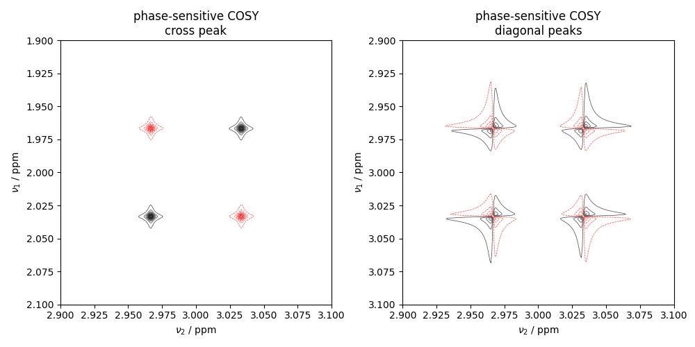
Zoom in on both the diagonal and the cross-peaks to better show peak shapes.

max_amp = phase_sensitive_COSY.real.max()
levels = np.linspace(-max_amp, max_amp, 30)  # levels from -max_amp to max_amp
options = dict(alpha=0.75, linewidths=0.5)  # plot options

# Separate positive and negative levels
positive_levels = levels[levels > 0]
negative_levels = levels[levels < 0]

fig, (ax1, ax2) = plt.subplots(1, 2, figsize=(10, 5), subplot_kw={"projection": "csdm"})

# Plot 1: Full view
ax1.contour(phase_sensitive_COSY.real, levels=positive_levels, colors="k", **options)
ax1.contour(phase_sensitive_COSY.real, levels=negative_levels, colors="r", **options)
ax1.invert_yaxis()
ax1.set_ylabel("$\\nu_1$ / ppm")
ax1.set_xlabel("$\\nu_2$ / ppm")
ax1.set_xlim(3.1, 2.9)
ax1.set_ylim(2.1, 1.9)
ax1.set_title("phase-sensitive COSY\ncross peak")
ax1.invert_xaxis()

# Plot 2: diagonal peak
ax2.contour(phase_sensitive_COSY.real, levels=positive_levels, colors="k", **options)
ax2.contour(phase_sensitive_COSY.real, levels=negative_levels, colors="r", **options)
ax2.invert_yaxis()
ax2.set_ylabel("$\\nu_1$ / ppm")
ax2.set_xlabel("$\\nu_2$ / ppm")
ax2.set_xlim(3.1, 2.9)
ax2.set_ylim(3.1, 2.9)
ax2.set_title("phase-sensitive COSY\ndiagonal peaks")
ax2.invert_xaxis()

plt.tight_layout()
plt.show()