Itraconazole, ¹³C (I=1/2) PASS¶

¹³C (I=1/2) 2D Phase-adjusted spinning sideband (PASS) simulation.

The following is a simulation of a 2D PASS spectrum of itraconazole, a triazole containing drug prescribed for the prevention and treatment of fungal infection. The 2D PASS spectrum is a correlation of finite speed MAS to an infinite speed MAS spectrum. The parameters for the simulation are obtained from Dey et al. [1].

import matplotlib.pyplot as plt

from mrsimulator import Simulator
from mrsimulator.method.lib import SSB2D
from mrsimulator import signal_processor as sp
from mrsimulator.method import SpectralDimension

There are 41 \(^{13}\text{C}\) single-site spin systems partially describing the NMR parameters of itraconazole. We will import the directly import the spin systems to the Simulator object using the load_spin_systems method.

sim = Simulator()

filename = "https://ssnmr.org/sites/default/files/mrsimulator/itraconazole_13C.mrsys"
sim.load_spin_systems(filename)

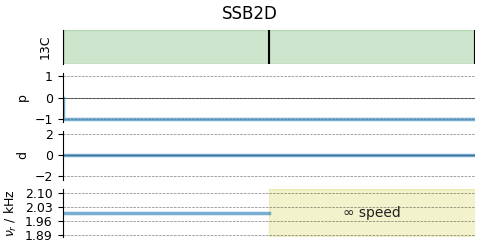
Use the SSB2D method to simulate a PASS, MAT, QPASS, QMAT, or any equivalent sideband separation spectrum. Here, we use the method to generate a PASS spectrum.

PASS = SSB2D(
    channels=["13C"],
    magnetic_flux_density=11.74,
    rotor_frequency=2000,
    spectral_dimensions=[
        SpectralDimension(
            count=20 * 4,
            spectral_width=2000 * 20,  # value in Hz
            label="Anisotropic dimension",
        ),
        SpectralDimension(
            count=1024,
            spectral_width=3e4,  # value in Hz
            reference_offset=1.1e4,  # value in Hz
            label="Isotropic dimension",
        ),
    ],
)
sim.methods = [PASS]  # add the method.

# A graphical representation of the method object.
plt.figure(figsize=(5, 2.5))
PASS.plot()
plt.show()

For 2D spinning sideband simulation, set the number of spinning sidebands in the Simulator.config object to spectral_width/rotor_frequency along the sideband dimension.

sim.config.number_of_sidebands = 20

# run the simulation.
sim.run()

Apply post-simulation processing. Here, we apply a Lorentzian line broadening to the isotropic dimension.

dataset = sim.methods[0].simulation
processor = sp.SignalProcessor(
    operations=[
        sp.IFFT(dim_index=0),
        sp.apodization.Exponential(FWHM="100 Hz", dim_index=0),
        sp.FFT(dim_index=0),
    ]
)
processed_dataset = processor.apply_operations(dataset=dataset).real
processed_dataset /= processed_dataset.max()

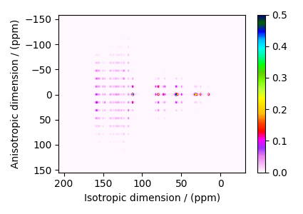
The plot of the simulation.

plt.figure(figsize=(4.25, 3.0))
ax = plt.subplot(projection="csdm")
cb = ax.imshow(processed_dataset, aspect="auto", cmap="gist_ncar_r", vmax=0.5)
plt.colorbar(cb)
ax.invert_xaxis()
ax.invert_yaxis()
plt.tight_layout()
plt.show()

Total running time of the script: ( 0 minutes 0.956 seconds)

Gallery generated by Sphinx-Gallery