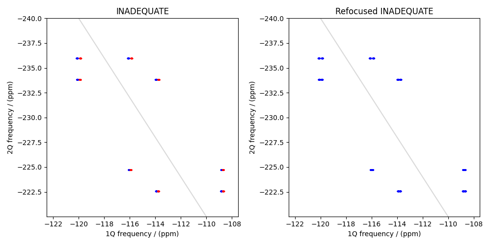
Sigma-2, ²⁹Si INADEQUATE and refocused INADEQUATE

²⁹Si INADEQUATE and refocused INADEQUATE simulation on Sigma-2

An example of the INADEQUATE and refocused INADEQUATE experiments on Sigma-2, a highly siliceous zeolite. We start by making all necessary imports.

from mrsimulator import Coupling, Site, SpinSystem, Method, Simulator
from mrsimulator.spin_system.isotope import Isotope
from mrsimulator.method import DelayEvent, MixingEvent, SpectralDimension, SpectralEvent
import mrsimulator.signal_processor as sp

import matplotlib.pyplot as plt
import numpy as np

Next, we build sites and couplings to describe Sigma-2

# 29Si chemical shifts for Sigma2
site_1 = Site(isotope="29Si", isotropic_chemical_shift=-115.97)
site_2 = Site(isotope="29Si", isotropic_chemical_shift=-113.82)
site_3 = Site(isotope="29Si", isotropic_chemical_shift=-119.98)
site_4 = Site(isotope="29Si", isotropic_chemical_shift=-108.73)

# 29Si J couplings for Sigma2
coupling_24 = Coupling(site_index=[0, 1], isotropic_j=12.16)
coupling_13 = Coupling(site_index=[0, 1], isotropic_j=20.5)
coupling_41 = Coupling(site_index=[0, 1], isotropic_j=9.48)
coupling_23 = Coupling(site_index=[0, 1], isotropic_j=16.6)

Now, we build spin systems to describe Sigma-2. Since Sigma-2 is a spin-dilute system, spins are either isolated (single-site systems) or next to only one other spin (two-site systems).

systems = [
    SpinSystem(sites=[site_1], abundance=3.85),
    SpinSystem(sites=[site_2], abundance=3.85),
    SpinSystem(sites=[site_3], abundance=3.85),
    SpinSystem(sites=[site_4], abundance=3.85),
    SpinSystem(sites=[site_2, site_4], couplings=[coupling_24], abundance=0.755),
    SpinSystem(sites=[site_1, site_3], couplings=[coupling_13], abundance=0.755),
    SpinSystem(sites=[site_1, site_4], couplings=[coupling_41], abundance=0.755),
    SpinSystem(sites=[site_2, site_3], couplings=[coupling_23], abundance=0.755),
]

Next, we calculate parameters that we will use in our method objects.

delay = 1 / (4 * coupling_23.isotropic_j)

B0 = Isotope(symbol="1H").ref_freq_to_B0(400 * 1e6)
Si29 = Isotope(symbol="29Si")

offset1Q = -115 * Si29.B0_to_ref_freq(B0) * 1e-6
offset2Q = -230 * Si29.B0_to_ref_freq(B0) * 1e-6

# zoom into the Site 2 and 4 region
sw1Q = 15 * Si29.B0_to_ref_freq(B0) * 1e-6
sw2Q = 20 * Si29.B0_to_ref_freq(B0) * 1e-6

We first build the INADEQUATE method

inadequate = Method(
    channels=["29Si"],
    magnetic_flux_density=B0,
    spectral_dimensions=[
        SpectralDimension(
            count=1024,
            spectral_width=sw2Q,
            reference_offset=offset2Q,
            label="2Q frequency",
            events=[
                DelayEvent(
                    duration=2 * delay,
                    freq_contrib=["J"],
                    transition_queries=[{"ch1": {"P": [-1]}}],
                ),
                MixingEvent(ch1={"angle": np.pi / 2}),
                SpectralEvent(
                    fraction=1, transition_queries=[{"ch1": {"P": [-1, -1]}}]
                ),
            ],
        ),
        SpectralDimension(
            count=1024,
            spectral_width=sw1Q,
            reference_offset=offset1Q,
            label="1Q frequency",
            events=[
                MixingEvent(ch1={"angle": np.pi / 2, "phase": np.pi / 2}),
                SpectralEvent(fraction=1, transition_queries=[{"ch1": {"P": [-1]}}]),
            ],
        ),
    ],
)

We also build the refocused INADEQUATE method

refocused_inadequate = Method(
    channels=["29Si"],
    magnetic_flux_density=B0,
    spectral_dimensions=[
        SpectralDimension(
            count=1024,
            spectral_width=sw2Q,
            reference_offset=offset2Q,
            label="2Q frequency",
            events=[
                DelayEvent(
                    duration=2 * delay,
                    freq_contrib=["J1_0"],
                    transition_queries=[{"ch1": {"P": [-1]}}],
                ),
                MixingEvent(ch1={"angle": np.pi / 2}),
                SpectralEvent(
                    fraction=1, transition_queries=[{"ch1": {"P": [-1, -1]}}]
                ),
            ],
        ),
        SpectralDimension(
            count=1024,
            spectral_width=sw1Q,
            reference_offset=offset1Q,
            label="1Q frequency",
            events=[
                MixingEvent(ch1={"angle": np.pi / 2}),
                DelayEvent(
                    duration=2 * delay,
                    freq_contrib=["J1_0"],
                    transition_queries=[{"ch1": {"P": [-1]}}],
                ),  # 2tau delay
                MixingEvent(),
                SpectralEvent(fraction=1, transition_queries=[{"ch1": {"P": [-1]}}]),
            ],
        ),
    ],
)

We now build the simulator, configure it, and run the simulation.

sim = Simulator(
    spin_systems=systems, methods=[inadequate, refocused_inadequate]
)  # , J_resolved
sim.config.integration_density = 1
sim.config.number_of_sidebands = 1
sim.run()

Next, we define the signal processor with apodization operations

apodizeINADEQUATE = sp.SignalProcessor(
    operations=[
        sp.IFFT(dim_index=(0, 1)),
        sp.apodization.Gaussian(FWHM="6 Hz", dim_index=0),
        sp.apodization.Gaussian(FWHM="3 Hz", dim_index=1),
        sp.FFT(dim_index=(0, 1)),
    ]
)

inadequate_spec = apodizeINADEQUATE.apply_operations(
    dataset=sim.methods[0].simulation
).real
inadequate_spec /= inadequate_spec.max()

refocused_inadequate_spec = apodizeINADEQUATE.apply_operations(
    dataset=sim.methods[1].simulation
).real
refocused_inadequate_spec /= refocused_inadequate_spec.max()

Lastly, we define levels for the contour plot and plot the results.

max_amp = inadequate_spec.real.max()

levels = np.linspace(-max_amp, max_amp, 40)  # levels from -max_amp to max_amp
options = dict(alpha=0.75, linewidths=0.5)  # plot options

# Separate positive and negative levels
positive_levels = levels[levels > 0]
negative_levels = levels[levels < 0]

fig, (ax1, ax2) = plt.subplots(1, 2, figsize=(10, 5), subplot_kw={"projection": "csdm"})

# Plot 1: INADEQUATE
ax1.contour(inadequate_spec.real, levels=positive_levels, colors="b")
ax1.contour(inadequate_spec.real, levels=negative_levels, colors="r")
ax1.plot([-130, -100], [-260, -200], color="k", alpha=0.15, label="y=2x")
ax1.invert_xaxis()
ax1.invert_yaxis()
ax1.set_title("INADEQUATE")
ax1.invert_xaxis()

# Plot 2: Refocused INADEQUATE
ax2.contour(refocused_inadequate_spec.real, levels=positive_levels, colors="b")
ax2.contour(refocused_inadequate_spec.real, levels=negative_levels, colors="r")
ax2.plot([-130, -100], [-260, -200], color="k", alpha=0.15, label="y=2x")
ax2.invert_xaxis()
ax2.invert_yaxis()
ax2.set_title("Refocused INADEQUATE")
ax2.invert_xaxis()

plt.tight_layout()
plt.show()