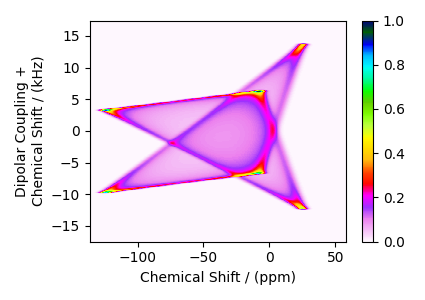
¹H 2D separated local field powder spectra

2D Simulation of polycrystalline methyl formate.

Equation (14) and (15) of the Linder et al. paper [1] are:

(41)\[\begin{split}\begin{align} \omega_1^{(1)}(\theta_r, \phi_r, \alpha, \beta) &= \omega_\text{cs}(\theta_r,\phi_r) + \frac{1}{\sqrt{3}} \omega_D(\theta_r,\phi_r,\alpha,\beta)\\ \omega_2^{(1)}(\theta_r, \phi_r, \alpha, \beta) &= \omega_\text{cs}(\theta_r,\phi_r) - \frac{1}{\sqrt{3}} \omega_D(\theta_r,\phi_r,\alpha,\beta), ~\text{and}\\ \omega^{(2)}(\theta_r, \phi_r) &= \omega_\text{cs}(\theta_r,\phi_r) \end{align}\end{split}\]

where \(\theta_r\) and \(\phi_r\) are the polar coordinates in the principal axis frame of the (asymmetric) nuclear shielding tensor, and \(\alpha\), \(\beta\) are the Euler angles required to orient the dipolar coupling tensor in the nuclear shielding principal axis frame defined with the Mehring convention. The scaling of the dipolar frequency contribution by \(1/\sqrt{3}\) is due to the use of off-resonance decoupling during the \(t_1\) period (see Fig. 1 of the paper).

The spin interaction tensor values for the carbonyl carbon of methyl formate (H-(C=O)-O-CH3) taken from the paper are \(\omega_d/(2 \pi) = 22,630\) Hz and \({\sigma_{1} = -126.6}\) ppm, \({\sigma_{2} = -7.0}\) ppm, and \({\sigma_{3} = 25.4}\) ppm using the Mehring convention. However, Mehring uses the symbol \(\sigma_{i}\) as the chemical shift values read off the spectrum. So, these values should be labeled \(\delta_{i}\).

Linder et al. use the term “chemical shielding” and the symbol sigma. The 2D plot dimensions are labeled as chemical shift.

In the Mehring convention, the principal components are ordered according to \(\sigma_{1}' \le \sigma_{2}' \le \sigma_{3}'\) where \(\sigma_{i}' =\sigma_{i} -\sigma_{\text{iso}}^{\text{ref}}\). The angle \(\beta\) is defined relative to the axis associated with \(\sigma_{3}'\). However, in the Haberlen convention this direction corresponds to the \(\lambda_{yy}\) direction. Therefore, we need to change the PAS angles for mrsimulator, which are defined relative to the \(\lambda_{zz}\) direction.

import matplotlib.pyplot as plt
import numpy as np

from mrsimulator import Simulator, SpinSystem, Site, Coupling
from mrsimulator.method import Method, SpectralDimension, SpectralEvent
from mrsimulator import signal_processor as sp
from mrsimulator.spin_system.tensors import SymmetricTensor
import mrsimulator.utils.cartesian_tensor as ct

D = 22630 * 1 / np.sqrt(3)  # Hz

delta_1 = -126.6  # ppm
delta_2 = -7.0  # ppm
delta_3 = 25.4  # ppm
delta_iso = (delta_1 + delta_2 + delta_3) / 3

mehring_eigenvalues = [-delta_1, -delta_2, -delta_3]  # in ppm
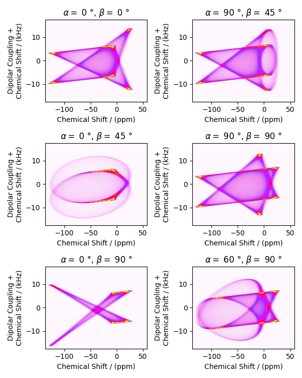
mehring_euler_angles = [
    (0, 0, 0),
    (0, -45, 0),
    (0, -90, 0),
    (-90, -45, 0),
    (-90, -90, 0),
    (-60, -90, 0),
]  # in degrees

# Convert angles to radians
mehring_euler_angles_rad = [
    (np.radians(alpha), np.radians(beta), np.radians(gamma))
    for alpha, beta, gamma in mehring_euler_angles
]

# Convert the tensor to Haeberlen parameters for each set of Euler angles
haeberlen_euler_angles = []
for euler_angle in mehring_euler_angles_rad:
    tensor = ct.from_mehring_params(
        euler_angles=euler_angle, eigenvalues=mehring_eigenvalues
    )
    euler_angles, zeta_sigma, eta_sigma, sigma_iso = ct.to_haeberlen_params(tensor)
    haeberlen_euler_angles.append(euler_angles)

/home/docs/checkouts/readthedocs.org/user_builds/mrsimulator/envs/stable/lib/python3.10/site-packages/sphinx_gallery/gen_rst.py:783: UserWarning: Gimbal lock detected. Setting third angle to zero since it is not possible to uniquely determine all angles.
  exec(self.code, self.fake_main.__dict__)

site1 = Site(
    isotope="1H",
    isotropic_chemical_shift=0,
)

# Create an empty list to store the spin_system objects
spin_systems = []

# Iterate through the list
for angles in haeberlen_euler_angles:
    alpha, beta, gamma = angles

    site2 = Site(
        isotope="13C",
        isotropic_chemical_shift=delta_iso,  # in ppm
        shielding_symmetric=SymmetricTensor(
            zeta=zeta_sigma, eta=eta_sigma, alpha=alpha, beta=beta, gamma=gamma
        ),
    )

    # Create a Coupling object for each set of Euler angles
    coupling = Coupling(
        site_index=[0, 1],
        dipolar=SymmetricTensor(D=D),  # D in Hz
    )

    # Add the Coupling object to the list
    spin_systems.append(SpinSystem(sites=[site1, site2], couplings=[coupling]))

slf = Method(
    channels=["13C"],
    magnetic_flux_density=2.4,  # in T
    rotor_angle=0,
    spectral_dimensions=[
        SpectralDimension(
            count=512,
            spectral_width=3.5e4,  # in Hz
            reference_offset=0,  # in Hz
            label="Dipolar Coupling +\nChemical Shift",
            events=[
                SpectralEvent(
                    transition_queries=[{"ch1": {"P": [-1]}}],
                    freq_contrib=["Shielding1_0", "Shielding1_2", "D1_2"],
                )
            ],
        ),
        SpectralDimension(
            count=512,
            spectral_width=5e3,  # in Hz
            reference_offset=-1e3,  # in Hz
            label="Chemical Shift",
            events=[
                SpectralEvent(
                    transition_queries=[{"ch1": {"P": [-1]}}],
                    freq_contrib=["Shielding1_0", "Shielding1_2"],
                )
            ],
        ),
    ],
)

Iterate through the list

simulations = []
times = []
for index, angles in enumerate(haeberlen_euler_angles):
    sim = Simulator(spin_systems=[spin_systems[index]], methods=[slf])
    sim.config.integration_volume = "hemisphere"
    sim.run()

    sim.methods[0].simulation.dimensions[1].to("kHz")
    simulations.append(sim)

processor = sp.SignalProcessor(
    operations=[
        # Gaussian convolution along both dimensions.
        sp.IFFT(dim_index=(0, 1)),
        sp.apodization.Gaussian(FWHM="0.15 kHz", dim_index=0),
        sp.apodization.Gaussian(FWHM="0.15 kHz", dim_index=1),
        sp.FFT(dim_index=(0, 1)),
    ]
)
processed_datasets = []
for index, angles in enumerate(haeberlen_euler_angles):
    processed_dataset = processor.apply_operations(
        dataset=simulations[index].methods[0].simulation
    )
    processed_dataset /= processed_dataset.max()
    processed_datasets.append(processed_dataset.real)

First plot

plt.figure(figsize=(4.25, 3.0))
ax = plt.subplot(projection="csdm")
cb = ax.imshow(
    processed_datasets[0] / processed_datasets[0].max(),
    aspect="auto",
    cmap="gist_ncar_r",
    interpolation="none",
)
plt.title(None)
plt.colorbar(cb)
plt.tight_layout()
plt.show()

All plots

fig, axs = plt.subplots(
    3, 2, figsize=(6, 7.5), subplot_kw={"projection": "csdm"}, tight_layout=True
)

index = 0
for j in range(2):
    for i in range(3):
        ax = axs[i, j]
        data = processed_datasets[index]
        cb = ax.imshow(data, aspect="auto", cmap="gist_ncar_r")
        # Get the corresponding Euler angles
        alpha, beta, gamma = mehring_euler_angles[index]
        # Set the title to include the Euler angles
        ax.set_title(f"$\\alpha=$ {-alpha} °, $\\beta=$ {-beta} °")
        index += 1

# Create a new axes for the colorbar at the specific position
cbar_ax = fig.add_axes([1, 0.07, 0.015, 0.23])
fig.colorbar(cb, cax=cbar_ax)
plt.show()

[1]

M. Linder, A. Höhener, and R. R. Ernst, Orientation of tensorial interactions determined from 2D NMR powder spectra, J. Chem. Phys. (1980) 73, 4959. DOI: 10.1063/5.0061611