Note
Go to the end to download the full example code.
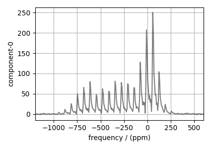
¹¹⁹Sn MAS NMR of SnO
The following is a spinning sideband manifold fitting example for the 119Sn MAS NMR of SnO. The dataset was acquired and shared by Altenhof et al. [1].
import csdmpy as cp
import numpy as np
import matplotlib.pyplot as plt
from lmfit import Minimizer

from mrsimulator import Simulator, SpinSystem, Site, Coupling
from mrsimulator.method.lib import BlochDecaySpectrum
from mrsimulator import signal_processor as sp
from mrsimulator.utils import spectral_fitting as sf
from mrsimulator.utils import get_spectral_dimensions
from mrsimulator.spin_system.tensors import SymmetricTensor
Import the dataset
filename = "https://ssnmr.org/sites/default/files/mrsimulator/119Sn_SnO.csdf"
experiment = cp.load(filename)

# For spectral fitting, we only focus on the real part of the complex dataset
experiment = experiment.real

# Convert the coordinates along each dimension from Hz to ppm.
_ = [item.to("ppm", "nmr_frequency_ratio") for item in experiment.dimensions]

# plot of the dataset.
plt.figure(figsize=(4.25, 3.0))
ax = plt.subplot(projection="csdm")
ax.plot(experiment, "k", alpha=0.5)
ax.set_xlim(-1200, 600)
plt.grid()
plt.tight_layout()
plt.show()
Estimate noise statistics from the dataset
coords = experiment.dimensions[0].coordinates
noise_region = np.where(coords > 300e-6)
noise_data = experiment[noise_region]

plt.figure(figsize=(3.75, 2.5))
ax = plt.subplot(projection="csdm")
ax.plot(noise_data, label="noise")
plt.title("Noise section")
plt.axis("off")
plt.tight_layout()
plt.show()

noise_mean, sigma = experiment[noise_region].mean(), experiment[noise_region].std()
noise_mean, sigma
(<Quantity 0.06896736>, <Quantity 0.67926073>)
Create a fitting model
Guess model
Create a guess list of spin systems. There are two spin systems present in this example, - 1) an uncoupled \(^{119}\text{Sn}\) and - 2) a coupled \(^{119}\text{Sn}\)-\(^{117}\text{Sn}\) spin systems.
sn119 = Site(
    isotope="119Sn",
    isotropic_chemical_shift=-210,
    shielding_symmetric=SymmetricTensor(zeta=700, eta=0.1),
)
sn117 = Site(
    isotope="117Sn",
    isotropic_chemical_shift=0,
)
j_sn = Coupling(
    site_index=[0, 1],
    isotropic_j=8150.0,
)

sn117_abundance = 7.68  # in %
spin_systems = [
    # uncoupled spin system
    SpinSystem(sites=[sn119], abundance=100 - sn117_abundance),
    # coupled spin systems
    SpinSystem(sites=[sn119, sn117], couplings=[j_sn], abundance=sn117_abundance),
]
Method
# Get the spectral dimension parameters from the experiment.
spectral_dims = get_spectral_dimensions(experiment)

MAS = BlochDecaySpectrum(
    channels=["119Sn"],
    magnetic_flux_density=9.395,  # in T
    rotor_frequency=10000,  # in Hz
    spectral_dimensions=spectral_dims,
    experiment=experiment,  # add the measurement to the method.
)
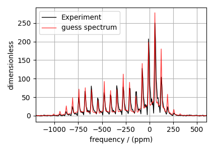
Guess Spectrum
# Simulation
# ----------
sim = Simulator(spin_systems=spin_systems, methods=[MAS])
sim.run()

# Post Simulation Processing
# --------------------------
processor = sp.SignalProcessor(
    operations=[
        sp.IFFT(),
        sp.apodization.Exponential(FWHM="1500 Hz"),
        sp.FFT(),
        sp.Scale(factor=50000),
    ]
)
processed_dataset = processor.apply_operations(dataset=sim.methods[0].simulation).real

# Plot of the guess Spectrum
# --------------------------
plt.figure(figsize=(4.25, 3.0))
ax = plt.subplot(projection="csdm")
ax.plot(experiment, "k", linewidth=1, label="Experiment")
ax.plot(processed_dataset, "r", alpha=0.75, linewidth=1, label="guess spectrum")
ax.set_xlim(-1200, 600)
plt.grid()
plt.legend()
plt.tight_layout()
plt.show()
Least-squares minimization with LMFIT
Use the make_LMFIT_params() for a quick
setup of the fitting parameters.
params = sf.make_LMFIT_params(sim, processor, include={"rotor_frequency"})

# Remove the abundance parameters from params. Since the measurement detects 119Sn, we
# also remove the isotropic chemical shift parameter of 117Sn site from params. The
# 117Sn is the site at index 1 of the spin system at index 1.
params.pop("sys_0_abundance")
params.pop("sys_1_abundance")
params.pop("sys_1_site_1_isotropic_chemical_shift")

# Since the 119Sn site is shared between the two spin systems, we add constraints to the
# 119Sn site parameters from the spin system at index 1 to be the same as 119Sn site
# parameters from the spin system at index 0.
lst = [
    "isotropic_chemical_shift",
    "shielding_symmetric_zeta",
    "shielding_symmetric_eta",
]
for item in lst:
    params[f"sys_1_site_0_{item}"].expr = f"sys_0_site_0_{item}"

print(params.pretty_print(columns=["value", "min", "max", "vary", "expr"]))
Name                                      Value      Min      Max     Vary     Expr
SP_0_operation_1_Exponential_FWHM          1500     -inf      inf     True     None
SP_0_operation_3_Scale_factor             5e+04     -inf      inf     True     None
mth_0_rotor_frequency                     1e+04     9900 1.01e+04     True     None
sys_0_site_0_isotropic_chemical_shift      -210     -inf      inf     True     None
sys_0_site_0_shielding_symmetric_eta        0.1        0        1     True     None
sys_0_site_0_shielding_symmetric_zeta       700     -inf      inf     True     None
sys_1_coupling_0_isotropic_j               8150     -inf      inf     True     None
sys_1_site_0_isotropic_chemical_shift      -210     -inf      inf    False sys_0_site_0_isotropic_chemical_shift
sys_1_site_0_shielding_symmetric_eta        0.1        0        1    False sys_0_site_0_shielding_symmetric_eta
sys_1_site_0_shielding_symmetric_zeta       700     -inf      inf    False sys_0_site_0_shielding_symmetric_zeta
None
Solve the minimizer using LMFIT
opt = sim.optimize()  # Pre-compute transition pathways
minner = Minimizer(
    sf.LMFIT_min_function,
    params,
    fcn_args=(sim, processor, sigma),
    fcn_kws={"opt": opt},
)
result = minner.minimize()
result
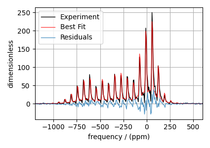
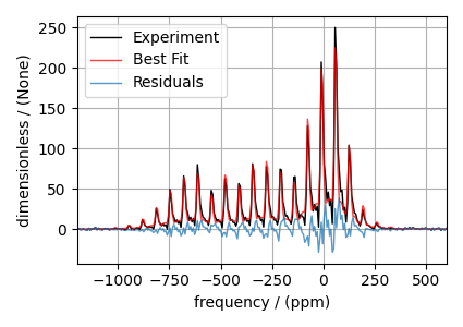
The best fit solution
best_fit = sf.bestfit(sim, processor)[0].real
residuals = sf.residuals(sim, processor)[0].real

# Plot the spectrum
plt.figure(figsize=(4.25, 3.0))
ax = plt.subplot(projection="csdm")
ax.plot(experiment, "k", linewidth=1, label="Experiment")
ax.plot(best_fit, "r", alpha=0.75, linewidth=1, label="Best Fit")
ax.plot(residuals, alpha=0.75, linewidth=1, label="Residuals")
ax.set_xlim(-1200, 600)
plt.grid()
plt.legend()
plt.tight_layout()
plt.show()
Total running time of the script: (0 minutes 2.648 seconds)