Simulate arbitrary transitions (single-quantum)

27Al (I=5/2) quadrupolar spectrum simulation.

The mrsimulator built-in one-dimensional methods, BlochDecaySpectrum and BlochDecayCentralTransitionSpectrum, are designed to simulate spectrum from all single quantum transitions or central transition selective transition, respectively. In this example, we show how you can simulate any arbitrary transition using the generic Method1D method.

import matplotlib as mpl
import matplotlib.pyplot as plt
from mrsimulator import Simulator, SpinSystem, Site
from mrsimulator.methods import Method1D

# global plot configuration
mpl.rcParams["figure.figsize"] = [4.5, 3.0]

Create a single-site arbitrary spin system.

site = Site(
    name="27Al",
    isotope="27Al",
    isotropic_chemical_shift=35.7,  # in ppm
    quadrupolar={"Cq": 5.959e6, "eta": 0.32},  # Cq is in Hz
)
spin_system = SpinSystem(sites=[site])

Selecting spin transitions for simulation

The arguments of the Method1D object are the same as the arguments of the BlochDecaySpectrum method; however, unlike a BlochDecaySpectrum method, the SpectralDimension object in Method1D contains additional argument—events.

The Event object is a collection of attributes, which are local to the event. It is here where we define a transition_query to select one or more transitions for simulating the spectrum. The two attributes of the transition_query are P and D, which are given as,

(3)\[\begin{split}P = m_f - m_i \\ D = m_f^2 - m_i^2,\end{split}\]

where \(m_f\) and \(m_i\) are the spin quantum numbers for the final and initial energy states. Based on the query, the method selects all transitions from the spin system that satisfy the query selection criterion. For example, to simulate a spectrum for the satellite transition, \(|-1/2\rangle\rightarrow|-3/2\rangle\), set the value of

(4)\[\begin{split}P &= (-3/2) - (-1/2) = -1 \\ D &= (9/4) - (1/4) = 2.\end{split}\]

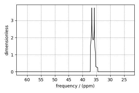
For illustrative purposes, let’s look at the infinite speed spectrum from this satellite transition.

method = Method1D(
    channels=["27Al"],
    magnetic_flux_density=21.14,  # in T
    rotor_frequency=1e9,  # in Hz
    spectral_dimensions=[
        {
            "count": 1024,
            "spectral_width": 1e4,  # in Hz
            "reference_offset": 1e4,  # in Hz
            "events": [
                {"transition_query": {"P": [-1], "D": [2]}}  # <-- select transitions
            ],
        }
    ],
)

Create the Simulator object and add the method and the spin system object.

sim = Simulator()
sim.spin_systems += [spin_system]  # add the spin system
sim.methods += [method]  # add the method

Simulate the spectrum.

sim.run()

# The plot of the simulation before signal processing.
ax = plt.subplot(projection="csdm")
ax.plot(sim.methods[0].simulation.real, color="black", linewidth=1)
ax.invert_xaxis()
plt.tight_layout()
plt.show()

Selecting both inner and outer-satellite transitions

You may use the same transition query selection criterion to select multiple transitions. Consider the following transitions with respective P and D values.

• \(|-1/2\rangle\rightarrow|-3/2\rangle\) (\(P=-1, D=2\))

• \(|-3/2\rangle\rightarrow|-5/2\rangle\) (\(P=-1, D=4\))

method2 = Method1D(
    channels=["27Al"],
    magnetic_flux_density=21.14,  # in T
    rotor_frequency=1e9,  # in Hz
    spectral_dimensions=[
        {
            "count": 1024,
            "spectral_width": 1e4,  # in Hz
            "reference_offset": 1e4,  # in Hz
            "events": [
                {"transition_query": {"P": [-1], "D": [2, 4]}}  # <-- select transitions
            ],
        }
    ],
)

Update the method object in the Simulator object.

sim.methods[0] = method2  # add the method

Simulate the spectrum.

sim.run()

# The plot of the simulation before signal processing.
ax = plt.subplot(projection="csdm")
ax.plot(sim.methods[0].simulation.real, color="black", linewidth=1)
ax.invert_xaxis()
plt.tight_layout()
plt.show()