Simulate arbitrary transitions (multi-quantum)

33S (I=5/2) quadrupolar spectrum simulation.

Simulate a triple quantum spectrum.

import matplotlib as mpl
import matplotlib.pyplot as plt
from mrsimulator import Simulator, SpinSystem, Site
from mrsimulator.methods import Method1D

# global plot configuration
mpl.rcParams["figure.figsize"] = [4.5, 3.0]

Create a single-site arbitrary spin system.

site = Site(
    name="27Al",
    isotope="27Al",
    isotropic_chemical_shift=35.7,  # in ppm
    quadrupolar={"Cq": 2.959e6, "eta": 0.98},  # Cq is in Hz
)
spin_system = SpinSystem(sites=[site])

Selecting the triple-quantum transition

For spin-site spin-5/2 spin system, there are three triple-quantum transition

• \(|1/2\rangle\rightarrow|-5/2\rangle\) (\(P=-3, D=6\))

• \(|3/2\rangle\rightarrow|-3/2\rangle\) (\(P=-3, D=0\))

• \(|5/2\rangle\rightarrow|-1/2\rangle\) (\(P=-3, D=-6\))

To select one or more triple-quantum transitions, assign the respective value of P and D to the transition_query.

method = Method1D(
    channels=["27Al"],
    magnetic_flux_density=21.14,  # in T
    rotor_frequency=1e9,  # in Hz
    spectral_dimensions=[
        {
            "count": 1024,
            "spectral_width": 5e3,  # in Hz
            "reference_offset": 2.5e4,  # in Hz
            "events": [
                {  # symmetric triple quantum transitions
                    "transition_query": {"P": [-3], "D": [0]}
                }
            ],
        }
    ],
)

Create the Simulator object and add the method and the spin system object.

sim = Simulator()
sim.spin_systems += [spin_system]  # add the spin system
sim.methods += [method]  # add the method
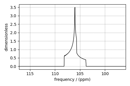
sim.run()

# The plot of the simulation before signal processing.
ax = plt.subplot(projection="csdm")
ax.plot(sim.methods[0].simulation.real, color="black", linewidth=1)
ax.invert_xaxis()
plt.tight_layout()
plt.show()