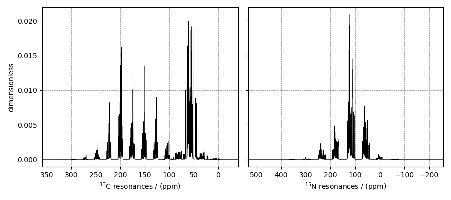
Protein GB1, 13C and 15N (I=1/2)

13C/15N (I=1/2) spinning sideband simulation.

The following is the spinning sideband simulation of a macromolecule, protein GB1. The \(^{13}\text{C}\) and \(^{15}\text{N}\) CSA tensor parameters were obtained from Hung et. al. 1, which consists of 42 \(^{13}\text{C}\alpha\), 44 \(^{13}\text{CO}\), and 44 \(^{15}\text{NH}\) tensors. In the following example, instead of creating 130 spin systems, we download the spin systems from a remote file and load it directly to the Simulator object.

import matplotlib as mpl
import matplotlib.pyplot as plt
import mrsimulator.signal_processing as sp
import mrsimulator.signal_processing.apodization as apo
from mrsimulator import Simulator
from mrsimulator.methods import BlochDecaySpectrum

# global plot configuration
mpl.rcParams["figure.figsize"] = [9, 4]

Create the Simulator object and load the spin systems from an external file.

sim = Simulator()

file_ = "https://sandbox.zenodo.org/record/687656/files/protein_GB1_15N_13CA_13CO.mrsys"
sim.load_spin_systems(file_)  # load the spin systems.
print(f"number of spin systems = {len(sim.spin_systems)}")

Out:

number of spin systems = 130

Create a \(^{13}\text{C}\) Bloch decay spectrum method.

method_13C = BlochDecaySpectrum(
    channels=["13C"],
    magnetic_flux_density=11.7,  # in T
    rotor_frequency=3000,  # in Hz
    spectral_dimensions=[
        {
            "count": 8192,
            "spectral_width": 5e4,  # in Hz
            "reference_offset": 2e4,  # in Hz
            "label": r"$^{13}$C resonances",
        }
    ],
)

Since the spin systems contain both \(^{13}\text{C}\) and \(^{15}\text{N}\) sites, let’s also create a \(^{15}\text{N}\) Bloch decay spectrum method.

method_15N = BlochDecaySpectrum(
    channels=["15N"],
    magnetic_flux_density=11.7,  # in T
    rotor_frequency=3000,  # in Hz
    spectral_dimensions=[
        {
            "count": 8192,
            "spectral_width": 4e4,  # in Hz
            "reference_offset": 7e3,  # in Hz
            "label": r"$^{15}$N resonances",
        }
    ],
)

Add the methods to the Simulator object and run the simulation

# Add the methods.
sim.methods = [method_13C, method_15N]

# Run the simulation.
sim.run()

# Get the simulation data from the respective methods.
data_13C = sim.methods[0].simulation  # method at index 0 is 13C Bloch decay method.
data_15N = sim.methods[1].simulation  # method at index 1 is 15N Bloch decay method.

Add post-simulation signal processing.

processor = sp.SignalProcessor(
    operations=[sp.IFFT(), apo.Exponential(FWHM="10 Hz"), sp.FFT()]
)
# apply post-simulation processing to data_13C
processed_data_13C = processor.apply_operations(data=data_13C).real

# apply post-simulation processing to data_15N
processed_data_15N = processor.apply_operations(data=data_15N).real

The plot of the simulation after signal processing.

fig, ax = plt.subplots(1, 2, subplot_kw={"projection": "csdm"}, sharey=True)

ax[0].plot(processed_data_13C, color="black", linewidth=0.5)
ax[0].invert_xaxis()

ax[1].plot(processed_data_15N, color="black", linewidth=0.5)
ax[1].set_ylabel(None)
ax[1].invert_xaxis()

plt.tight_layout()
plt.show()

1

Hung I., Ge Y., Liu X., Liu M., Li C., Gan Z., Measuring \(^{13}\text{C}\)/\(^{15}\text{N}\) chemical shift anisotropy in [\(^{13}\text{C}\), \(^{15}\text{N}\)] uniformly enriched proteins using CSA amplification, Solid State Nuclear Magnetic Resonance. 2015, 72, 96-103. DOI: 10.1016/j.ssnmr.2015.09.002