Czjzek distribution (Shielding and Quadrupolar)

In this example, we illustrate the simulation of spectrum originating from a Czjzek distribution of traceless symmetric tensors. We show two cases, the Czjzek distribution of the shielding and quadrupolar tensor parameters, respectively.

Import the required modules.

import matplotlib as mpl
import matplotlib.pyplot as plt
import numpy as np
from mrsimulator import Simulator
from mrsimulator.methods import BlochDecaySpectrum, BlochDecayCentralTransitionSpectrum
from mrsimulator.models import CzjzekDistribution
from mrsimulator.utils.collection import single_site_system_generator

# pre config the figures
mpl.rcParams["figure.figsize"] = [4.25, 3.0]

Symmetric shielding tensor

Create the Czjzek distribution

First, create a distribution of the zeta and eta parameters of the shielding tensors using the Czjzek distribution model as follows.

# The range of zeta and eta coordinates over which the distribution is sampled.
z_range = np.arange(100) - 50  # in ppm
e_range = np.arange(21) / 20
z_dist, e_dist, amp = CzjzekDistribution(sigma=3.1415).pdf(pos=[z_range, e_range])

Here z_range and e_range are the coordinates along the \(\zeta\) and \(\eta\) dimensions that form a two-dimensional \(\zeta\)-\(\eta\) grid. The argument sigma of the CzjzekDistribution class is the standard deviation of the second-rank tensor parameters used in generating the distribution, and pos hold the one-dimensional arrays of \(\zeta\) and \(\eta\) coordinates, respectively.

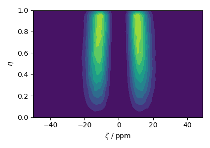
The following is the contour plot of the Czjzek distribution.

plt.contourf(z_dist, e_dist, amp, levels=10)
plt.xlabel(r"$\zeta$ / ppm")
plt.ylabel(r"$\eta$")
plt.tight_layout()
plt.show()

Simulate the spectrum

To quickly generate single-site spin systems from the above \(\zeta\) and \(\eta\) parameters, use the single_site_system_generator() utility function.

systems = single_site_system_generator(
    isotopes="13C", shielding_symmetric={"zeta": z_dist, "eta": e_dist}, abundance=amp
)

Here, the variable systems hold an array of single-site spin systems. Next, create a simulator object and add the above system and a method.

sim = Simulator()
sim.spin_systems = systems  # add the systems
sim.methods = [BlochDecaySpectrum(channels=["13C"])]  # add the method
sim.run()

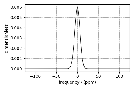
The following is the static spectrum arising from a Czjzek distribution of the second-rank traceless shielding tensors.

plt.figure(figsize=(4.5, 3.0))
ax = plt.gca(projection="csdm")
ax.plot(sim.methods[0].simulation, color="black", linewidth=1)
plt.tight_layout()
plt.show()

Quadrupolar tensor

Create the Czjzek distribution

Similarly, you may also create a Czjzek distribution of the electric field gradient (EFG) tensor parameters.

# The range of Cq and eta coordinates over which the distribution is sampled.
cq_range = np.arange(100) * 0.6 - 30  # in MHz
e_range = np.arange(21) / 20
cq_dist, e_dist, amp = CzjzekDistribution(sigma=2.3).pdf(pos=[cq_range, e_range])

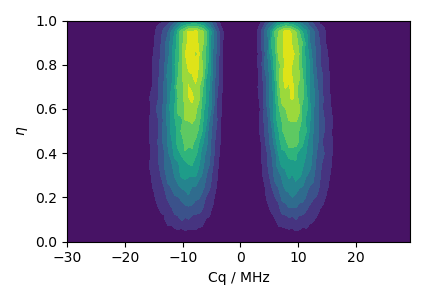
# The following is the contour plot of the Czjzek distribution.
plt.contourf(cq_dist, e_dist, amp, levels=10)
plt.xlabel(r"Cq / MHz")
plt.ylabel(r"$\eta$")
plt.tight_layout()
plt.show()

Simulate the spectrum

Create the spin systems.

systems = single_site_system_generator(
    isotopes="71Ga", quadrupolar={"Cq": cq_dist * 1e6, "eta": e_dist}, abundance=amp
)

Create a simulator object and add the above system.

sim = Simulator()
sim.spin_systems = systems  # add the systems
sim.methods = [
    BlochDecayCentralTransitionSpectrum(
        channels=["71Ga"],
        magnetic_flux_density=4.8,  # in T
        spectral_dimensions=[{"count": 2048, "spectral_width": 1.2e6}],
    )
]  # add the method
sim.run()

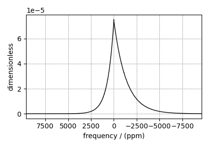
The following is the static spectrum arising from a Czjzek distribution of the second-rank traceless EFG tensors.

plt.figure(figsize=(4.25, 3.0))
ax = plt.gca(projection="csdm")
ax.plot(sim.methods[0].simulation, color="black", linewidth=1)
ax.invert_xaxis()
plt.tight_layout()
plt.show()