Extended Czjzek distribution (Shielding and Quadrupolar)

In this example, we illustrate the simulation of spectrum originating from an extended Czjzek distribution of traceless symmetric tensors. We show two cases, an extended Czjzek distribution of the shielding and quadrupolar tensor parameters, respectively.

Import the required modules.

import matplotlib as mpl
import matplotlib.pyplot as plt
import numpy as np
from mrsimulator import Simulator
from mrsimulator.methods import BlochDecaySpectrum, BlochDecayCentralTransitionSpectrum
from mrsimulator.models import ExtCzjzekDistribution
from mrsimulator.utils.collection import single_site_system_generator

# pre config the figures
mpl.rcParams["figure.figsize"] = [4.25, 3.0]

Symmetric shielding tensor

Create the extended Czjzek distribution

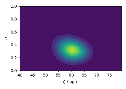
First, create a distribution of the zeta and eta parameters of the shielding tensors using the Extended Czjzek distribution model as follows,

# The range of zeta and eta coordinates over which the distribution is sampled.
z_lim = np.arange(100) * 0.4 + 40  # in ppm
e_lim = np.arange(21) / 20

dominant = {"zeta": 60, "eta": 0.3}
z_dist, e_dist, amp = ExtCzjzekDistribution(dominant, eps=0.14).pdf(pos=[z_lim, e_lim])

The following is the plot of the extended Czjzek distribution.

plt.contourf(z_dist, e_dist, amp, levels=10)
plt.xlabel(r"$\zeta$ / ppm")
plt.ylabel(r"$\eta$")
plt.tight_layout()
plt.show()

Simulate the spectrum

Create the spin systems from the above \(\zeta\) and \(\eta\) parameters.

systems = single_site_system_generator(
    isotopes="13C", shielding_symmetric={"zeta": z_dist, "eta": e_dist}, abundance=amp
)
print(len(systems))

Out:

838

Create a simulator object and add the above system.

sim = Simulator()
sim.spin_systems = systems  # add the systems
sim.methods = [BlochDecaySpectrum(channels=["13C"])]  # add the method
sim.run()

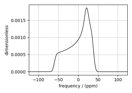
The following is the static spectrum arising from a Czjzek distribution of the second-rank traceless shielding tensors.

plt.figure(figsize=(4.25, 3.0))
ax = plt.gca(projection="csdm")
ax.plot(sim.methods[0].simulation, color="black", linewidth=1)
plt.tight_layout()
plt.show()

Quadrupolar tensor

Create the extended Czjzek distribution

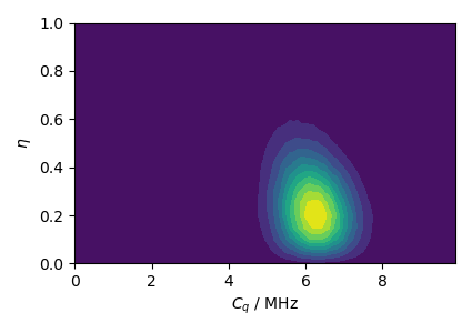
Similarly, you may also create an extended Czjzek distribution of the electric field gradient (EFG) tensor parameters.

# The range of Cq and eta coordinates over which the distribution is sampled.
cq_lim = np.arange(100) * 0.1  # assumed in MHz
e_lim = np.arange(21) / 20

dominant = {"Cq": 6.1, "eta": 0.1}
cq_dist, e_dist, amp = ExtCzjzekDistribution(dominant, eps=0.25).pdf(
    pos=[cq_lim, e_lim]
)

The following is the plot of the extended Czjzek distribution.

plt.contourf(cq_dist, e_dist, amp, levels=10)
plt.xlabel(r"$C_q$ / MHz")
plt.ylabel(r"$\eta$")
plt.tight_layout()
plt.show()

Simulate the spectrum

Static spectrum Create the spin systems.

systems = single_site_system_generator(
    isotopes="71Ga", quadrupolar={"Cq": cq_dist * 1e6, "eta": e_dist}, abundance=amp
)

Create a simulator object and add the above system.

sim = Simulator()
sim.spin_systems = systems  # add the systems
sim.methods = [
    BlochDecayCentralTransitionSpectrum(
        channels=["71Ga"],
        magnetic_flux_density=9.4,  # in T
        spectral_dimensions=[{"count": 2048, "spectral_width": 2e5}],
    )
]  # add the method
sim.run()

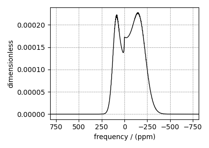
The following is a static spectrum arising from an extended Czjzek distribution of the second-rank traceless EFG tensors.

plt.figure(figsize=(4.25, 3.0))
ax = plt.gca(projection="csdm")
ax.plot(sim.methods[0].simulation, color="black", linewidth=1)
ax.invert_xaxis()
plt.tight_layout()
plt.show()

MAS spectrum

sim.methods = [
    BlochDecayCentralTransitionSpectrum(
        channels=["71Ga"],
        magnetic_flux_density=9.4,  # in T
        rotor_frequency=25000,  # in Hz
        spectral_dimensions=[
            {"count": 2048, "spectral_width": 2e5, "reference_offset": -1e4}
        ],
    )
]  # add the method
sim.config.number_of_sidebands = 16
sim.run()

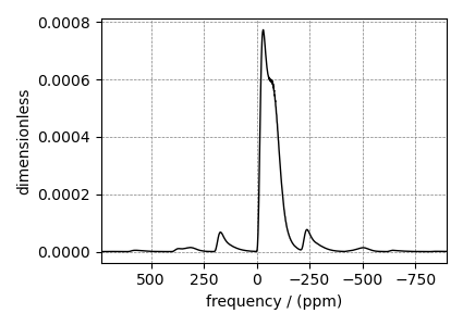
The following is the MAS spectrum arising from an extended Czjzek distribution of the second-rank traceless EFG tensors.

plt.figure(figsize=(4.25, 3.0))
ax = plt.gca(projection="csdm")
ax.plot(sim.methods[0].simulation, color="black", linewidth=1)
ax.invert_xaxis()
plt.tight_layout()
plt.show()