Albite, 27Al (I=5/2) 3QMAS

27Al (I=5/2) triple-quantum magic-angle spinning (3Q-MAS) simulation.

The following is an example of \(^{27}\text{Al}\) 3QMAS simulation of albite \(\text{NaSi}_3\text{AlO}_8\). The \(^{27}\text{Al}\) tensor parameters were obtained from Massiot et. al. 1.

import matplotlib as mpl
import matplotlib.pyplot as plt
import mrsimulator.signal_processing as sp
import mrsimulator.signal_processing.apodization as apo
from mrsimulator import Simulator, SpinSystem, Site
from mrsimulator.methods import ThreeQ_VAS

# global plot configuration
font = {"size": 9}
mpl.rc("font", **font)
mpl.rcParams["figure.figsize"] = [4.25, 3.0]

Generate the site and spin system objects.

site = Site(
    isotope="27Al",
    isotropic_chemical_shift=64.7,  # in ppm
    quadrupolar={"Cq": 3.25e6, "eta": 0.68},  # Cq is in Hz
)

spin_systems = [SpinSystem(sites=[site])]

Select a Triple Quantum variable-angle spinning method. You may optionally provide a rotor_angle to the method. The default rotor_angle is the magic-angle.

method = ThreeQ_VAS(
    channels=["27Al"],
    magnetic_flux_density=7,  # in T
    spectral_dimensions=[
        {
            "count": 256,
            "spectral_width": 1e4,  # in Hz
            "reference_offset": -3e3,  # in Hz
            "label": "Isotropic dimension",
        },
        {
            "count": 512,
            "spectral_width": 1e4,  # in Hz
            "reference_offset": 4e3,  # in Hz
            "label": "MAS dimension",
        },
    ],
)

Create the Simulator object, add the method and spin system objects, and run the simulation.

sim = Simulator()
sim.spin_systems = spin_systems  # add the spin systems
sim.methods = [method]  # add the method.
sim.run()

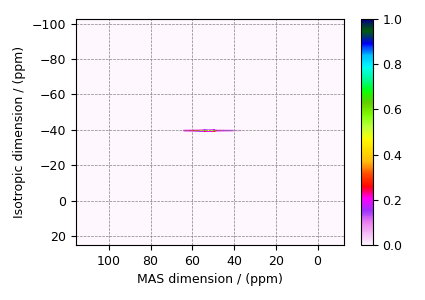
The plot of the simulation.

data = sim.methods[0].simulation
ax = plt.subplot(projection="csdm")
cb = ax.imshow(data / data.max(), aspect="auto", cmap="gist_ncar_r")
plt.colorbar(cb)
ax.invert_xaxis()
ax.invert_yaxis()
plt.tight_layout()
plt.show()

Add post-simulation signal processing.

processor = sp.SignalProcessor(
    operations=[
        # Gaussian convolution along both dimensions.
        sp.IFFT(dim_index=(0, 1)),
        apo.Gaussian(FWHM="0.2 kHz", dim_index=0),
        apo.Gaussian(FWHM="0.2 kHz", dim_index=1),
        sp.FFT(dim_index=(0, 1)),
    ]
)
processed_data = processor.apply_operations(data=sim.methods[0].simulation)
processed_data /= processed_data.max()

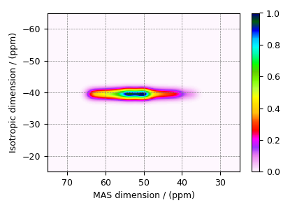
The plot of the simulation after signal processing.

ax = plt.subplot(projection="csdm")
cb = ax.imshow(processed_data.real, cmap="gist_ncar_r", aspect="auto")
plt.colorbar(cb)
ax.set_xlim(75, 25)
ax.set_ylim(-15, -65)
plt.tight_layout()
plt.show()

1

Massiot, D., Touzoa, B., Trumeaua, D., Coutures, J.P., Virlet, J., Florian, P., Grandinetti, P.J. Two-dimensional magic-angle spinning isotropic reconstruction sequences for quadrupolar nuclei, ssnmr, (1996), 6, 1, 73-83. DOI: 10.1016/0926-2040(95)01210-9