RbNO3, 87Rb (I=3/2) STMAS

87Rb (I=3/2) staellite-transition off magic-angle spinning simulation.

The following is an example of the STMAS simulation of \(\text{RbNO}_3\). The \(^{87}\text{Rb}\) tensor parameters were obtained from Massiot et. al. 1.

import matplotlib as mpl
import matplotlib.pyplot as plt
import mrsimulator.signal_processing as sp
import mrsimulator.signal_processing.apodization as apo
from mrsimulator import Simulator, SpinSystem, Site
from mrsimulator.methods import ST1_VAS

# global plot configuration
font = {"size": 9}
mpl.rc("font", **font)
mpl.rcParams["figure.figsize"] = [4.25, 3.0]

Generate the site and spin system objects.

Rb87_1 = Site(
    isotope="87Rb",
    isotropic_chemical_shift=-27.4,  # in ppm
    quadrupolar={"Cq": 1.68e6, "eta": 0.2},  # Cq is in Hz
)
Rb87_2 = Site(
    isotope="87Rb",
    isotropic_chemical_shift=-28.5,  # in ppm
    quadrupolar={"Cq": 1.94e6, "eta": 1.0},  # Cq is in Hz
)
Rb87_3 = Site(
    isotope="87Rb",
    isotropic_chemical_shift=-31.3,  # in ppm
    quadrupolar={"Cq": 1.72e6, "eta": 0.5},  # Cq is in Hz
)

sites = [Rb87_1, Rb87_2, Rb87_3]  # all sites
spin_systems = [SpinSystem(sites=[s]) for s in sites]

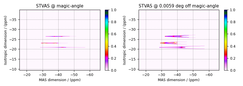
Step 2: Select a satellite-transition variable-angle spinning method. The following ST1_VAS method correlates the frequencies from the two inner-satellite transitions to the central transition. Note, STMAS measurements are highly suspectable to rotor angle mismatch. In the following, we show two methods, first set to magic-angle and the second deliberately miss-sets by approximately 0.0059 degrees.

angles = [54.7359, 54.73]
method = []
for angle in angles:
    method.append(
        ST1_VAS(
            channels=["87Rb"],
            magnetic_flux_density=7,  # in T
            rotor_angle=angle * 3.14159 / 180,  # in rad (magic angle)
            spectral_dimensions=[
                {
                    "count": 256,
                    "spectral_width": 3e3,  # in Hz
                    "reference_offset": -2.4e3,  # in Hz
                    "label": "Isotropic dimension",
                },
                {
                    "count": 512,
                    "spectral_width": 5e3,  # in Hz
                    "reference_offset": -4e3,  # in Hz
                    "label": "MAS dimension",
                },
            ],
        )
    )

Create the Simulator object, add the method and spin system objects, and run the simulation.

sim = Simulator()
sim.spin_systems = spin_systems  # add the spin systems
sim.methods = method  # add the methods.
sim.run()

The plot of the simulation.

data = [sim.methods[0].simulation, sim.methods[1].simulation]
fig, ax = plt.subplots(1, 2, figsize=(8.5, 3), subplot_kw={"projection": "csdm"})

titles = ["STVAS @ magic-angle", "STVAS @ 0.0059 deg off magic-angle"]
for i, item in enumerate(data):
    cb1 = ax[i].imshow(item / item.max(), aspect="auto", cmap="gist_ncar_r")
    ax[i].set_title(titles[i])
    plt.colorbar(cb1, ax=ax[i])
    ax[i].invert_xaxis()
    ax[i].invert_yaxis()
plt.tight_layout()
plt.show()

Add post-simulation signal processing.

processor = sp.SignalProcessor(
    operations=[
        # Gaussian convolution along both dimensions.
        sp.IFFT(dim_index=(0, 1)),
        apo.Gaussian(FWHM="50 Hz", dim_index=0),
        apo.Gaussian(FWHM="50 Hz", dim_index=1),
        sp.FFT(dim_index=(0, 1)),
    ]
)
processed_data = []
for item in data:
    processed_data.append(processor.apply_operations(data=item))
    processed_data[-1] /= processed_data[-1].max()

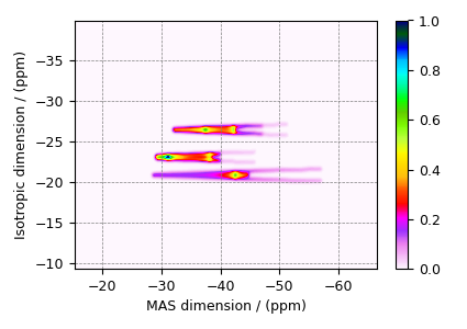
The plot of the simulation after signal processing.

ax = plt.subplot(projection="csdm")
cb = ax.imshow(processed_data[1].real, cmap="gist_ncar_r", aspect="auto")
plt.colorbar(cb)
ax.invert_xaxis()
ax.invert_yaxis()
plt.tight_layout()
plt.show()

1

Massiot, D., Touzoa, B., Trumeaua, D., Coutures, J.P., Virlet, J., Florian, P., Grandinetti, P.J. Two-dimensional magic-angle spinning isotropic reconstruction sequences for quadrupolar nuclei, ssnmr, (1996), 6, 1, 73-83. DOI: 10.1016/0926-2040(95)01210-9