Czjzek distribution, 27Al (I=5/2) 3QMAS

27Al (I=5/2) 3QMAS simulation of amorphous material.

In this section, we illustrate the simulation of a quadrupolar MQMAS spectrum arising from a distribution of the electric field gradient (EFG) tensors from amorphous material. We proceed by employing the Czjzek distribution model.

import matplotlib as mpl
import matplotlib.pyplot as plt
import numpy as np
from mrsimulator import Simulator
from mrsimulator.methods import ThreeQ_VAS
from mrsimulator.models import CzjzekDistribution
from mrsimulator.utils.collection import single_site_system_generator
from scipy.stats import multivariate_normal

# global plot configuration
mpl.rcParams["figure.figsize"] = [4.5, 3.0]

Generate probability distribution

# The range of isotropic chemical shifts, the quadrupolar coupling constant, and
# asymmetry parameters used in generating a 3D grid.
iso_r = np.arange(101) / 1.5 + 30  # in ppm
Cq_r = np.arange(100) / 4  # in MHz
eta_r = np.arange(10) / 9

# The 3D mesh grid over which the distribution amplitudes are evaluated.
iso, Cq, eta = np.meshgrid(iso_r, Cq_r, eta_r, indexing="ij")

# The 2D amplitude grid of Cq and eta is sampled from the Czjzek distribution model.
Cq_dist, e_dist, amp = CzjzekDistribution(sigma=1).pdf(pos=[Cq_r, eta_r])

# The 1D amplitude grid of isotropic chemical shifts is sampled from a Gaussian model.
iso_amp = multivariate_normal(mean=58, cov=[4]).pdf(iso_r)

# The 3D amplitude grid is generated as an uncorrelated distribution of the above two
# distribution, which is the product of the two distributions.
pdf = np.repeat(amp, iso_r.size).reshape(eta_r.size, Cq_r.size, iso_r.size)
pdf *= iso_amp
pdf = pdf.T

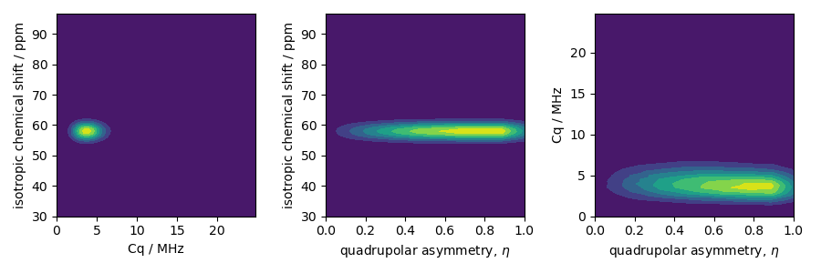
The two-dimensional projections from this three-dimensional distribution are shown below.

_, ax = plt.subplots(1, 3, figsize=(9, 3))

# isotropic shift v.s. quadrupolar coupling constant
ax[0].contourf(Cq_r, iso_r, pdf.sum(axis=2))
ax[0].set_xlabel("Cq / MHz")
ax[0].set_ylabel("isotropic chemical shift / ppm")

# isotropic shift v.s. quadrupolar asymmetry
ax[1].contourf(eta_r, iso_r, pdf.sum(axis=1))
ax[1].set_xlabel(r"quadrupolar asymmetry, $\eta$")
ax[1].set_ylabel("isotropic chemical shift / ppm")

# quadrupolar coupling constant v.s. quadrupolar asymmetry
ax[2].contourf(eta_r, Cq_r, pdf.sum(axis=0))
ax[2].set_xlabel(r"quadrupolar asymmetry, $\eta$")
ax[2].set_ylabel("Cq / MHz")

plt.tight_layout()
plt.show()

Simulation setup

Let’s create the site and spin system objects from these parameters. Use the single_site_system_generator() utility function to generate single-site spin systems.

spin_systems = single_site_system_generator(
    isotopes="27Al",
    isotropic_chemical_shifts=iso,
    quadrupolar={"Cq": Cq * 1e6, "eta": eta},  # Cq in Hz
    abundance=pdf,
)
len(spin_systems)

Out:

5770

Simulate a \(^{27}\text{Al}\) 3Q-MAS spectrum by using the ThreeQ_MAS method.

mqvas = ThreeQ_VAS(
    channels=["27Al"],
    spectral_dimensions=[
        {
            "count": 512,
            "spectral_width": 26718.475776,  # in Hz
            "reference_offset": -4174.76184,  # in Hz
            "label": "Isotropic dimension",
        },
        {
            "count": 512,
            "spectral_width": 2e4,  # in Hz
            "reference_offset": 2e3,  # in Hz
            "label": "MAS dimension",
        },
    ],
)

Create the simulator object, add the spin systems and method, and run the simulation.

sim = Simulator()
sim.spin_systems = spin_systems  # add the spin systems
sim.methods = [mqvas]  # add the method
sim.config.number_of_sidebands = 1
sim.run()

data = sim.methods[0].simulation

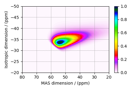
The plot of the corresponding spectrum.

ax = plt.subplot(projection="csdm")
cb = ax.imshow(data / data.max(), cmap="gist_ncar_r", aspect="auto")
plt.colorbar(cb)
ax.set_ylim(-20, -50)
ax.set_xlim(80, 20)
plt.tight_layout()
plt.show()