Simulating site disorder (crystalline)

87Rb (I=3/2) 3QMAS simulation with site disorder.

The following example illustrates an NMR simulation of a crystalline solid with site disorders. We model such disorders with Extended Czjzek distribution. The following case study shows an \(^{87}\text{Rb}\) 3QMAS simulation of RbNO3.

import matplotlib as mpl
import numpy as np
from mrsimulator import Simulator
from mrsimulator.methods import ThreeQ_VAS
import matplotlib.pyplot as plt

from mrsimulator.models import ExtCzjzekDistribution
from mrsimulator.utils.collection import single_site_system_generator
from scipy.stats import multivariate_normal

# global plot configuration
mpl.rcParams["figure.figsize"] = [4.5, 3.0]

Generate probability distribution

Create three extended Czjzek distributions for the three sites in RbNO3 about their respective mean tensors.

# The range of isotropic chemical shifts, the quadrupolar coupling constant, and
# asymmetry parameters used in generating a 3D grid.
iso_r = np.arange(101) / 6.5 - 35  # in ppm
Cq_r = np.arange(100) / 100 + 1.25  # in MHz
eta_r = np.arange(11) / 10

# The 3D mesh grid over which the distribution amplitudes are evaluated.
iso, Cq, eta = np.meshgrid(iso_r, Cq_r, eta_r, indexing="ij")


def get_prob_dist(iso, Cq, eta, eps, cov):
    pdf = 0
    for i in range(len(iso)):
        # The 2D amplitudes for Cq and eta is sampled from the extended Czjzek model.
        avg_tensor = {"Cq": Cq[i], "eta": eta[i]}
        _, _, amp = ExtCzjzekDistribution(avg_tensor, eps=eps[i]).pdf(pos=[Cq_r, eta_r])

        # The 1D amplitudes for isotropic chemical shifts is sampled as a Gaussian.
        iso_amp = multivariate_normal(mean=iso[i], cov=[cov[i]]).pdf(iso_r)

        # The 3D amplitude grid is generated as an uncorrelated distribution of the
        # above two distribution, which is the product of the two distributions.
        pdf_t = np.repeat(amp, iso_r.size).reshape(eta_r.size, Cq_r.size, iso_r.size)
        pdf_t *= iso_amp
        pdf += pdf_t
    return pdf


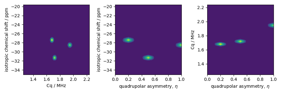
iso_0 = [-27.4, -28.5, -31.3]  # isotropic chemical shifts for the three sites in ppm
Cq_0 = [1.68, 1.94, 1.72]  # Cq in MHz for the three sites
eta_0 = [0.2, 1, 0.5]  # eta for the three sites
eps_0 = [0.02, 0.02, 0.02]  # perturbation fractions for extended Czjzek distribution.
var_0 = [0.1, 0.1, 0.1]  # variance for the isotropic chemical shifts in ppm^2.

pdf = get_prob_dist(iso_0, Cq_0, eta_0, eps_0, var_0).T

The two-dimensional projections from this three-dimensional distribution are shown below.

_, ax = plt.subplots(1, 3, figsize=(9, 3))

# isotropic shift v.s. quadrupolar coupling constant
ax[0].contourf(Cq_r, iso_r, pdf.sum(axis=2))
ax[0].set_xlabel("Cq / MHz")
ax[0].set_ylabel("isotropic chemical shift / ppm")

# isotropic shift v.s. quadrupolar asymmetry
ax[1].contourf(eta_r, iso_r, pdf.sum(axis=1))
ax[1].set_xlabel(r"quadrupolar asymmetry, $\eta$")
ax[1].set_ylabel("isotropic chemical shift / ppm")

# quadrupolar coupling constant v.s. quadrupolar asymmetry
ax[2].contourf(eta_r, Cq_r, pdf.sum(axis=0))
ax[2].set_xlabel(r"quadrupolar asymmetry, $\eta$")
ax[2].set_ylabel("Cq / MHz")
plt.tight_layout()
plt.show()

Simulation setup

Generate spin systems from the above probability distribution.

spin_systems = single_site_system_generator(
    isotopes="87Rb",
    isotropic_chemical_shifts=iso,
    quadrupolar={"Cq": Cq * 1e6, "eta": eta},  # Cq in Hz
    abundance=pdf,
)
len(spin_systems)

Out:

510

Simulate a \(^{27}\text{Al}\) 3Q-MAS spectrum by using the ThreeQ_MAS method.

method = ThreeQ_VAS(
    channels=["87Rb"],
    magnetic_flux_density=9.4,  # in T
    rotor_angle=54.735 * np.pi / 180,
    spectral_dimensions=[
        {
            "count": 96,
            "spectral_width": 7e3,  # in Hz
            "reference_offset": -7e3,  # in Hz
            "label": "Isotropic dimension",
        },
        {
            "count": 256,
            "spectral_width": 1e4,  # in Hz
            "reference_offset": -4e3,  # in Hz
            "label": "MAS dimension",
        },
    ],
)

Create the simulator object, add the spin systems and method, and run the simulation.

sim = Simulator()
sim.spin_systems = spin_systems  # add the spin systems
sim.methods = [method]  # add the method
sim.config.number_of_sidebands = 1
sim.run()

data = sim.methods[0].simulation

The plot of the corresponding spectrum.

ax = plt.subplot(projection="csdm")
cb = ax.imshow(data / data.max(), cmap="gist_ncar_r", aspect="auto")
ax.set_ylim(-40, -70)
ax.set_xlim(-20, -60)
plt.colorbar(cb)
plt.tight_layout()
plt.show()