Fitting Cusipidine

After acquiring an NMR spectrum, we often require a least-squares analysis to determine site populations and nuclear spin interaction parameters. Generally, this comprises of two steps:

• create a fitting model, and

• determine the model parameters that give the best fit to the spectrum.

Here, we will use the mrsimulator objects to create a fitting model, and use the LMFIT library for performing the least-squares fitting optimization. In this example, we use a synthetic \(^{29}\text{Si}\) NMR spectrum of cuspidine, generated from the tensor parameters reported by Hansen et. al. 1, to demonstrate a simple fitting procedure.

We will begin by importing relevant modules and establishing figure size.

import csdmpy as cp
import matplotlib as mpl
import matplotlib.pyplot as plt
import mrsimulator.signal_processing as sp
import mrsimulator.signal_processing.apodization as apo
from mrsimulator import Simulator, SpinSystem
from mrsimulator.methods import BlochDecaySpectrum
from lmfit import Minimizer, Parameters, fit_report

font = {"size": 9}
mpl.rc("font", **font)
mpl.rcParams["figure.figsize"] = [4.5, 3.0]

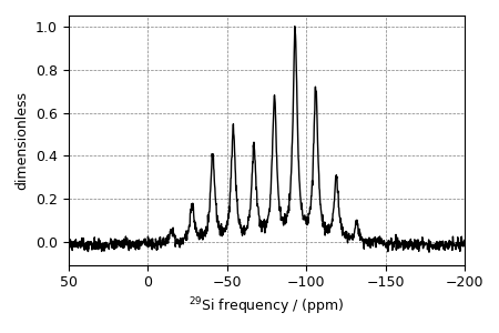
Import the dataset

Use the csdmpy module to load the synthetic dataset as a CSDM object.

file_ = "https://sandbox.zenodo.org/record/687656/files/synthetic_cuspidine_test.csdf"
synthetic_experiment = cp.load(file_)

# convert the dimension coordinates from Hz to ppm
synthetic_experiment.dimensions[0].to("ppm", "nmr_frequency_ratio")

# Normalize the spectrum
synthetic_experiment /= synthetic_experiment.max()

# Plot of the synthetic dataset.
ax = plt.subplot(projection="csdm")
ax.plot(synthetic_experiment, color="black", linewidth=1)
ax.set_xlim(-200, 50)
ax.invert_xaxis()
plt.tight_layout()
plt.show()

Create a fitting model

Before you can fit a simulation to an experiment, in this case, the synthetic dataset, you will first need to create a fitting model. We will use the mrsimulator objects as tools in creating a model for the least-squares fitting.

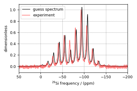
Step 1: Create initial guess sites and spin systems. The initial guess is often based on some prior knowledge about the system under investigation. For the current example, we know that Cuspidine is a crystalline silica polymorph with one crystallographic Si site. Therefore, our initial guess model is a single \(^{29}\text{Si}\) site spin system. For non-linear fitting algorithms, as a general recommendation, the initial guess model parameters should be a good starting point for the algorithms to converge.

# the guess model comprising of a single site spin system
site = dict(
    isotope="29Si",
    isotropic_chemical_shift=-82.0,  # in ppm,
    shielding_symmetric={"zeta": -63, "eta": 0.4},  # zeta in ppm
)

system_object = SpinSystem(
    name="Si Site",
    description="A 29Si site in cuspidine",
    sites=[site],  # from the above code
    abundance=100,
)

Step 2: Create the method object. The method should be the same as the one used in the measurement. In this example, we use the BlochDecaySpectrum method. Note, when creating the method object, the value of the method parameters must match the respective values used in the experiment.

method = BlochDecaySpectrum(
    channels=["29Si"],
    magnetic_flux_density=7.1,  # in T
    rotor_frequency=780,  # in Hz
    spectral_dimensions=[
        {
            "count": 2048,
            "spectral_width": 25000,  # in Hz
            "reference_offset": -5000,  # in Hz
        }
    ],
)

Step 3: Create the Simulator object and add the method and spin system objects.

sim = Simulator()
sim.spin_systems = [system_object]
sim.methods = [method]

sim.methods[0].experiment = synthetic_experiment

Step 5: Simulate the spectrum.

sim.run()

Step 6: Create a SignalProcessor class and apply post simulation processing.

processor = sp.SignalProcessor(
    operations=[
        sp.IFFT(),
        apo.Exponential(FWHM="200 Hz"),
        sp.FFT(),
        sp.Scale(factor=1.5),
    ]
)
processed_data = processor.apply_operations(data=sim.methods[0].simulation)

Step 7: The plot the spectrum. We also plot the synthetic dataset for comparison.

ax = plt.subplot(projection="csdm")
ax.plot(processed_data.real, c="k", linewidth=1, label="guess spectrum")
ax.plot(synthetic_experiment.real, c="r", linewidth=1.5, alpha=0.5, label="experiment")
ax.set_xlim(-200, 50)
ax.invert_xaxis()
plt.legend()
plt.tight_layout()
plt.show()

Setup a Least-squares minimization

Now that our model is ready, the next step is to set up a least-squares minimization. You may use any optimization package of choice, here we show an application using LMFIT. You may read more on the LMFIT documentation page.

Create fitting parameters

Next, you will need a list of parameters that will be used in the fit. The LMFIT library provides a Parameters class to create a list of parameters.

site1 = system_object.sites[0]
params = Parameters()

params.add(name="iso", value=site1.isotropic_chemical_shift)
params.add(name="eta", value=site1.shielding_symmetric.eta, min=0, max=1)
params.add(name="zeta", value=site1.shielding_symmetric.zeta)
params.add(name="FWHM", value=processor.operations[1].FWHM)
params.add(name="factor", value=processor.operations[3].factor)

Create a minimization function

Note, the above set of parameters does not know about the model. You will need to set up a function that will

• update the parameters of the Simulator and SignalProcessor object based on the LMFIT parameter updates,

• re-simulate the spectrum based on the updated values, and

• return the difference between the experiment and simulation.

def minimization_function(params, sim, processor):
    values = params.valuesdict()

    # the experiment data as a Numpy array
    intensity = sim.methods[0].experiment.dependent_variables[0].components[0].real

    # Here, we update simulation parameters iso, eta, and zeta for the site object
    site = sim.spin_systems[0].sites[0]
    site.isotropic_chemical_shift = values["iso"]
    site.shielding_symmetric.eta = values["eta"]
    site.shielding_symmetric.zeta = values["zeta"]

    # run the simulation
    sim.run()

    # update the SignalProcessor parameter and apply line broadening.
    # update the scaling factor parameter at index 3 of operations list.
    processor.operations[3].factor = values["factor"]
    # update the exponential apodization FWHM parameter at index 1 of operations list.
    processor.operations[1].FWHM = values["FWHM"]

    # apply signal processing
    processed_data = processor.apply_operations(sim.methods[0].simulation)

    # return the difference vector.
    return intensity - processed_data.dependent_variables[0].components[0].real

Note

To automate the fitting process, we provide a function to parse the Simulator and SignalProcessor objects for parameters and construct an LMFIT Parameters object. Similarly, a minimization function, analogous to the above minimization_function, is also included in the mrsimulator library. See the next example for usage instructions.

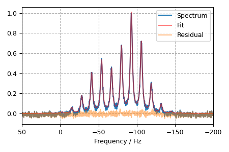
Perform the least-squares minimization

With the synthetic dataset, simulation, and the initial guess parameters, we are ready to perform the fit. To fit, we use the LMFIT Minimizer class.

minner = Minimizer(minimization_function, params, fcn_args=(sim, processor))
result = minner.minimize()
print(fit_report(result))

Out:

[[Fit Statistics]]
    # fitting method   = leastsq
    # function evals   = 43
    # data points      = 2048
    # variables        = 5
    chi-square         = 0.64652669
    reduced chi-square = 3.1646e-04
    Akaike info crit   = -16498.4360
    Bayesian info crit = -16470.3129
[[Variables]]
    iso:    -79.9380013 +/- 0.00711831 (0.01%) (init = -82)
    eta:     0.59954040 +/- 0.00454110 (0.76%) (init = 0.4)
    zeta:   -57.8375715 +/- 0.14157932 (0.24%) (init = -63)
    FWHM:    190.132207 +/- 1.05980445 (0.56%) (init = 200)
    factor:  1.36785444 +/- 0.00530840 (0.39%) (init = 1.5)
[[Correlations]] (unreported correlations are < 0.100)
    C(FWHM, factor) =  0.531
    C(eta, zeta)    =  0.321
    C(zeta, factor) = -0.228
    C(eta, factor)  =  0.165

The plot of the fit, measurement and the residuals is shown below.

plt.figsize = (4, 3)
x, y_data = synthetic_experiment.to_list()
residual = result.residual
plt.plot(x, y_data, label="Spectrum")
plt.plot(x, y_data - residual, "r", alpha=0.5, label="Fit")
plt.plot(x, residual, alpha=0.5, label="Residual")

plt.xlabel("Frequency / Hz")
plt.xlim(-200, 50)
plt.gca().invert_xaxis()
plt.grid(which="major", axis="both", linestyle="--")
plt.legend()
plt.tight_layout()
plt.show()

1

Hansen, M. R., Jakobsen, H. J., Skibsted, J., \(^{29}\text{Si}\) Chemical Shift Anisotropies in Calcium Silicates from High-Field \(^{29}\text{Si}\) MAS NMR Spectroscopy, Inorg. Chem. 2003, 42, 7, 2368-2377. DOI: 10.1021/ic020647f