Fitting 17O MAS NMR of crystalline Na2SiO3

In this example, we illustrate the use of the mrsimulator objects to

• create a spin system fitting model,

• use the fitting model to perform a least-squares fit on the experimental, and

• extract the tensor parameters of the spin system model.

We will be using the LMFIT methods to establish fitting parameters and fit the spectrum. The following example illustrates the least-squares fitting on a \(^{17}\text{O}\) measurement of \(\text{Na}_{2}\text{SiO}_{3}\) 1.

We will begin by importing relevant modules and presetting figure style and layout.

import csdmpy as cp
import matplotlib as mpl
import matplotlib.pyplot as plt
import mrsimulator.signal_processing as sp
import mrsimulator.signal_processing.apodization as apo
from lmfit import Minimizer, report_fit
from mrsimulator import Simulator, SpinSystem, Site
from mrsimulator.methods import BlochDecayCentralTransitionSpectrum
from mrsimulator.utils import get_spectral_dimensions
from mrsimulator.utils.spectral_fitting import LMFIT_min_function, make_LMFIT_params

font = {"size": 9}
mpl.rc("font", **font)
mpl.rcParams["figure.figsize"] = [4.25, 3.0]

Import the dataset

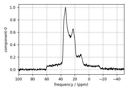
Import the experimental data. In this example, we will import the dataset file serialized with the CSDM file-format, using the csdmpy module.

filename = "https://sandbox.zenodo.org/record/687656/files/Na2SiO3_O17.csdf"
oxygen_experiment = cp.load(filename)

# For spectral fitting, we only focus on the real part of the complex dataset
oxygen_experiment = oxygen_experiment.real

# Convert the dimension coordinates from Hz to ppm.
oxygen_experiment.dimensions[0].to("ppm", "nmr_frequency_ratio")

# Normalize the spectrum
oxygen_experiment /= oxygen_experiment.max()

# plot of the dataset.
ax = plt.subplot(projection="csdm")
ax.plot(oxygen_experiment, color="black", linewidth=1)
ax.set_xlim(-50, 100)
ax.invert_xaxis()
plt.tight_layout()
plt.show()

Create a fitting model

Next, we will create a simulator object that we use to fit the spectrum. We will start by creating the guess SpinSystem objects.

Step 1: Create initial guess sites and spin systems

O17_1 = Site(
    isotope="17O",
    isotropic_chemical_shift=60.0,  # in ppm,
    quadrupolar={"Cq": 4.2e6, "eta": 0.5},  # Cq in Hz
)

O17_2 = Site(
    isotope="17O",
    isotropic_chemical_shift=40.0,  # in ppm,
    quadrupolar={"Cq": 2.4e6, "eta": 0},  # Cq in Hz
)

system_object = [SpinSystem(sites=[s], abundance=50) for s in [O17_1, O17_2]]

Step 2: Create the method object. Note, when performing the least-squares fit, you must create an appropriate method object which matches the method used in acquiring the experimental data. The attribute values of this method must match the exact conditions under which the experiment was acquired. This including the acquisition channels, the magnetic flux density, rotor angle, rotor frequency, and the spectral/spectroscopic dimension. In the following example, we set up a central transition selective Bloch decay spectrum method, where we obtain the spectral/spectroscopic information from the metadata of the CSDM dimension. Use the get_spectral_dimensions() utility function for quick extraction of the spectroscopic information, i.e., count, spectral_width, and reference_offset from the CSDM object. The remaining attribute values are set to the experimental conditions.

# get the count, spectral_width, and reference_offset information from the experiment.
spectral_dims = get_spectral_dimensions(oxygen_experiment)

method = BlochDecayCentralTransitionSpectrum(
    channels=["17O"],
    magnetic_flux_density=9.4,  # in T
    rotor_frequency=14000,  # in Hz
    spectral_dimensions=spectral_dims,
)

Assign the experimental dataset to the experiment attribute of the above method.

method.experiment = oxygen_experiment

Step 3: Create the Simulator object and add the method and spin system objects.

sim = Simulator()
sim.spin_systems = system_object
sim.methods = [method]

Step 4: Simulate the spectrum.

for iso in sim.spin_systems:
    # A method object queries every spin system for a list of transition pathways that
    # are relevant for the given method. Since the method and the number of spin systems
    # remain the same during the least-squares fit, a one-time query is sufficient. To
    # avoid querying for the transition pathways at every iteration in a least-squares
    # fitting, evaluate the transition pathways once and store it as follows
    iso.transition_pathways = method.get_transition_pathways(iso)

# Now simulate as usual.
sim.run()

Step 5: Create the SignalProcessor class object and apply the post-simulation signal processing operations.

processor = sp.SignalProcessor(
    operations=[
        sp.IFFT(),
        apo.Gaussian(FWHM="100 Hz"),
        sp.FFT(),
        sp.Scale(factor=20000.0),
    ]
)
processed_data = processor.apply_operations(data=sim.methods[0].simulation)

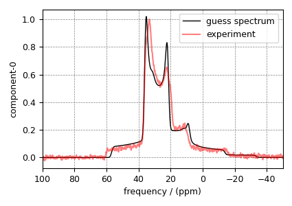
Step 6: The plot of initial guess simulation (black) along with the experiment (red) is shown below.

ax = plt.subplot(projection="csdm")
ax.plot(processed_data.real, color="black", linewidth=1, label="guess spectrum")
ax.plot(oxygen_experiment, c="r", linewidth=1.5, alpha=0.5, label="experiment")
ax.set_xlim(-50, 100)
ax.invert_xaxis()
plt.legend()
plt.tight_layout()
plt.show()

Least-squares minimization with LMFIT

Once you have a fitting model, you need to create the list of parameters to use in the least-squares fitting. For this, you may use the Parameters class from LMFIT, as described in the previous example. Here, we make use of a utility function, make_LMFIT_params(), that considerably simplifies the LMFIT parameters generation process.

Step 7: Create a list of parameters.

params = make_LMFIT_params(sim, processor)

The make_LMFIT_params parses the instances of the Simulator and the PostSimulator objects for parameters and returns an LMFIT Parameters object.

Customize the Parameters: You may customize the parameters list, params, as desired. Here, we remove the abundance of the two spin systems and constrain it to the initial value of 50% each.

params.pop("sys_0_abundance")
params.pop("sys_1_abundance")
params.pretty_print()

Out:

Name                                      Value      Min      Max   Stderr     Vary     Expr Brute_Step
operation_1_Gaussian_FWHM                   100     -inf      inf     None     True     None     None
operation_3_Scale_factor                  2e+04     -inf      inf     None     True     None     None
sys_0_site_0_isotropic_chemical_shift        60     -inf      inf     None     True     None     None
sys_0_site_0_quadrupolar_Cq             4.2e+06     -inf      inf     None     True     None     None
sys_0_site_0_quadrupolar_eta                0.5        0        1     None     True     None     None
sys_1_site_0_isotropic_chemical_shift        40     -inf      inf     None     True     None     None
sys_1_site_0_quadrupolar_Cq             2.4e+06     -inf      inf     None     True     None     None
sys_1_site_0_quadrupolar_eta                  0        0        1     None     True     None     None

Step 8: Perform least-squares minimization. For the user’s convenience, we also provide a utility function, LMFIT_min_function(), for evaluating the difference vector between the simulation and experiment, based on the parameters update. You may use this function directly as the argument of the LMFIT Minimizer class, as follows,

minner = Minimizer(LMFIT_min_function, params, fcn_args=(sim, processor))
result = minner.minimize()
report_fit(result)

Out:

[[Fit Statistics]]
    # fitting method   = leastsq
    # function evals   = 75
    # data points      = 4096
    # variables        = 8
    chi-square         = 1.47285018
    reduced chi-square = 3.6029e-04
    Akaike info crit   = -32467.6014
    Bayesian info crit = -32417.0593
[[Variables]]
    sys_0_site_0_isotropic_chemical_shift:  63.1644543 +/- 0.15646429 (0.25%) (init = 60)
    sys_0_site_0_quadrupolar_Cq:            4255845.06 +/- 7374.39734 (0.17%) (init = 4200000)
    sys_0_site_0_quadrupolar_eta:           0.52688815 +/- 0.00416758 (0.79%) (init = 0.5)
    sys_1_site_0_isotropic_chemical_shift:  39.3214919 +/- 0.06149227 (0.16%) (init = 40)
    sys_1_site_0_quadrupolar_Cq:            2399432.05 +/- 6060.12351 (0.25%) (init = 2400000)
    sys_1_site_0_quadrupolar_eta:           0.00460343 +/- 0.06747584 (1465.77%) (init = 0)
    operation_1_Gaussian_FWHM:              176.197353 +/- 1.70616109 (0.97%) (init = 100)
    operation_3_Scale_factor:               21407.0797 +/- 47.5123039 (0.22%) (init = 20000)
[[Correlations]] (unreported correlations are < 0.100)
    C(sys_1_site_0_isotropic_chemical_shift, sys_1_site_0_quadrupolar_Cq)           =  0.978
    C(sys_1_site_0_quadrupolar_Cq, sys_1_site_0_quadrupolar_eta)                    =  0.938
    C(sys_1_site_0_isotropic_chemical_shift, sys_1_site_0_quadrupolar_eta)          =  0.931
    C(sys_0_site_0_isotropic_chemical_shift, sys_0_site_0_quadrupolar_Cq)           =  0.903
    C(sys_0_site_0_quadrupolar_eta, sys_1_site_0_isotropic_chemical_shift)          =  0.438
    C(sys_0_site_0_quadrupolar_eta, sys_1_site_0_quadrupolar_Cq)                    =  0.375
    C(sys_0_site_0_quadrupolar_Cq, operation_3_Scale_factor)                        =  0.363
    C(sys_0_site_0_isotropic_chemical_shift, operation_3_Scale_factor)              =  0.337
    C(sys_0_site_0_quadrupolar_Cq, sys_0_site_0_quadrupolar_eta)                    = -0.307
    C(sys_0_site_0_quadrupolar_eta, operation_1_Gaussian_FWHM)                      = -0.298
    C(operation_1_Gaussian_FWHM, operation_3_Scale_factor)                          =  0.286
    C(sys_0_site_0_quadrupolar_Cq, sys_1_site_0_isotropic_chemical_shift)           = -0.277
    C(sys_1_site_0_quadrupolar_eta, operation_1_Gaussian_FWHM)                      =  0.263
    C(sys_0_site_0_quadrupolar_eta, sys_1_site_0_quadrupolar_eta)                   =  0.256
    C(sys_0_site_0_quadrupolar_Cq, sys_1_site_0_quadrupolar_Cq)                     = -0.243
    C(sys_0_site_0_isotropic_chemical_shift, operation_1_Gaussian_FWHM)             =  0.235
    C(sys_0_site_0_quadrupolar_Cq, operation_1_Gaussian_FWHM)                       =  0.201
    C(sys_0_site_0_isotropic_chemical_shift, sys_1_site_0_isotropic_chemical_shift) = -0.197
    C(sys_0_site_0_quadrupolar_Cq, sys_1_site_0_quadrupolar_eta)                    = -0.188
    C(sys_0_site_0_isotropic_chemical_shift, sys_0_site_0_quadrupolar_eta)          = -0.175
    C(sys_0_site_0_isotropic_chemical_shift, sys_1_site_0_quadrupolar_Cq)           = -0.159
    C(sys_1_site_0_quadrupolar_Cq, operation_1_Gaussian_FWHM)                       =  0.156
    C(sys_1_site_0_isotropic_chemical_shift, operation_1_Gaussian_FWHM)             =  0.122

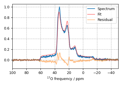
Step 9: The plot of the fit, measurement and the residuals is shown below.

plt.figsize = (4, 3)
x, y_data = oxygen_experiment.to_list()
residual = result.residual
plt.plot(x, y_data, label="Spectrum")
plt.plot(x, y_data - residual, "r", alpha=0.5, label="Fit")
plt.plot(x, residual, alpha=0.5, label="Residual")

plt.xlabel("$^{17}$O frequency / ppm")
plt.xlim(-50, 100)
plt.gca().invert_xaxis()
plt.grid(which="major", axis="both", linestyle="--")
plt.legend()
plt.tight_layout()
plt.show()

1

T. M. Clark, P. Florian, J. F. Stebbins, and P. J. Grandinetti, An \(^{17}\text{O}\) NMR Investigation of Crystalline Sodium Metasilicate: Implications for the Determination of Local Structure in Alkali Silicates, J. Phys. Chem. B. 2001, 105, 12257-12265. DOI: 10.1021/jp011289p