
Note
Click here to download the full example code or to run this example in your browser via Binder
17O DAS NMR of Coesite
Coesite is a high-pressure (2-3 GPa) and high-temperature (700°C) polymorph of silicon dioxide \(\text{SiO}_2\). Coesite has five crystallographic \(^{17}\text{O}\) sites. The experimental dataset used in this example is published in Grandinetti et. al. 1
import numpy as np
import csdmpy as cp
import matplotlib as mpl
import matplotlib.pyplot as plt
import mrsimulator.signal_processing as sp
import mrsimulator.signal_processing.apodization as apo
from mrsimulator import Simulator
from mrsimulator.methods import Method2D
from mrsimulator.utils import get_spectral_dimensions
from mrsimulator.utils.collection import single_site_system_generator
from mrsimulator.utils.spectral_fitting import LMFIT_min_function, make_LMFIT_params
from lmfit import Minimizer, report_fit


# global plot configuration
mpl.rcParams["figure.figsize"] = [4.5, 3.0]
Import the dataset
filename = "https://sandbox.zenodo.org/record/687656/files/DASCoesite.csdf"
experiment = cp.load(filename)
# For spectral fitting, we only focus on the real part of the complex dataset
experiment = experiment.real
# Convert the coordinates along each dimension from Hz to ppm.
_ = [item.to("ppm", "nmr_frequency_ratio") for item in experiment.dimensions]
# Normalize the spectrum
experiment /= experiment.max()
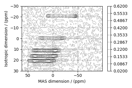
# plot of the dataset.
levels = (np.arange(10) + 0.3) / 15 # contours are drawn at these levels.
ax = plt.subplot(projection="csdm")
cb = ax.contour(experiment, colors="k", levels=levels, alpha=0.5, linewidths=0.5)
plt.colorbar(cb)
ax.invert_xaxis()
ax.set_ylim(30, -30)
plt.tight_layout()
plt.show()
Create a fitting model
The fitting model includes the Simulator and SignalProcessor objects. First, create the Simulator object.
# Create the guess sites and spin systems.
# default unit of isotropic_chemical_shift is ppm and Cq is Hz.
shifts = [29, 41, 57, 53, 58]  # in ppm
Cq = [6.1e6, 5.4e6, 5.5e6, 5.5e6, 5.1e6]  # in  Hz
eta = [0.1, 0.2, 0.1, 0.1, 0.3]
abundance = [1, 1, 2, 2, 2]

spin_systems = single_site_system_generator(
    isotopes="17O",
    isotropic_chemical_shifts=shifts,
    quadrupolar={"Cq": Cq, "eta": eta},
    abundance=abundance,
)

# Create the DAS method.
# Get the spectral dimension paramters from the experiment.
spectral_dims = get_spectral_dimensions(experiment)
das = Method2D(
    channels=["17O"],
    magnetic_flux_density=11.7,  # in T
    spectral_dimensions=[
        {
            **spectral_dims[0],
            "events": [
                {"fraction": 0.5, "rotor_angle": 37.38 * 3.14159 / 180},
                {"fraction": 0.5, "rotor_angle": 79.19 * 3.14159 / 180},
            ],
        },
        # The last spectral dimension block is the direct-dimension
        {**spectral_dims[1], "events": [{"rotor_angle": 54.735 * 3.14159 / 180}]},
    ],
    experiment=experiment,  # also add the measurement to the method.
)

# Optimize the script by pre-setting the transition pathways for each spin system from
# the das method.
for sys in spin_systems:
    sys.transition_pathways = das.get_transition_pathways(sys)
# Add Post simulation processing.
processor = sp.SignalProcessor(
    operations=[
        # Gaussian convolution along both dimensions.
        sp.IFFT(dim_index=(0, 1)),
        apo.Gaussian(FWHM="0.15 kHz", dim_index=0),
        apo.Gaussian(FWHM="0.15 kHz", dim_index=1),
        sp.FFT(dim_index=(0, 1)),
        sp.Scale(factor=1 / 8),
    ]
)
# Apply post simulation operations.
processed_data = processor.apply_operations(data=sim.methods[0].simulation).real
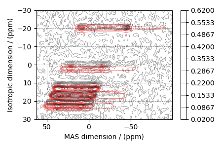
# The plot of the simulation after signal processing.
ax = plt.subplot(projection="csdm")
ax.contour(processed_data, colors="r", levels=levels, alpha=0.75, linewidths=0.5)
cb = ax.contour(experiment, colors="k", levels=levels, alpha=0.5, linewidths=0.5)
plt.colorbar(cb)
ax.invert_xaxis()
ax.set_ylim(30, -30)
plt.tight_layout()
plt.show()
Least-squares minimization with LMFIT
First, create the fitting parameters.
Use the make_LMFIT_params() for a quick
setup.
params = make_LMFIT_params(sim, processor)

# Here, we fix the abundance parameters to their initial value.
for i in range(5):
    params[f"sys_{i}_abundance"].vary = False

params.pretty_print()
Out:
Name                                      Value      Min      Max   Stderr     Vary     Expr Brute_Step
operation_1_Gaussian_FWHM                  0.15     -inf      inf     None     True     None     None
operation_2_Gaussian_FWHM                  0.15     -inf      inf     None     True     None     None
operation_4_Scale_factor                  0.125     -inf      inf     None     True     None     None
sys_0_abundance                            12.5        0      100     None    False     None     None
sys_0_site_0_isotropic_chemical_shift        29     -inf      inf     None     True     None     None
sys_0_site_0_quadrupolar_Cq             6.1e+06     -inf      inf     None     True     None     None
sys_0_site_0_quadrupolar_eta                0.1        0        1     None     True     None     None
sys_1_abundance                            12.5        0      100     None    False     None     None
sys_1_site_0_isotropic_chemical_shift        41     -inf      inf     None     True     None     None
sys_1_site_0_quadrupolar_Cq             5.4e+06     -inf      inf     None     True     None     None
sys_1_site_0_quadrupolar_eta                0.2        0        1     None     True     None     None
sys_2_abundance                              25        0      100     None    False     None     None
sys_2_site_0_isotropic_chemical_shift        57     -inf      inf     None     True     None     None
sys_2_site_0_quadrupolar_Cq             5.5e+06     -inf      inf     None     True     None     None
sys_2_site_0_quadrupolar_eta                0.1        0        1     None     True     None     None
sys_3_abundance                              25        0      100     None    False     None     None
sys_3_site_0_isotropic_chemical_shift        53     -inf      inf     None     True     None     None
sys_3_site_0_quadrupolar_Cq             5.5e+06     -inf      inf     None     True     None     None
sys_3_site_0_quadrupolar_eta                0.1        0        1     None     True     None     None
sys_4_abundance                              25        0      100     None    False 100-sys_0_abundance-sys_1_abundance-sys_2_abundance-sys_3_abundance     None
sys_4_site_0_isotropic_chemical_shift        58     -inf      inf     None     True     None     None
sys_4_site_0_quadrupolar_Cq             5.1e+06     -inf      inf     None     True     None     None
sys_4_site_0_quadrupolar_eta                0.3        0        1     None     True     None     None
Run the minimization using LMFIT
minner = Minimizer(LMFIT_min_function, params, fcn_args=(sim, processor))
result = minner.minimize()
report_fit(result)
Out:
[[Fit Statistics]]
    # fitting method   = leastsq
    # function evals   = 371
    # data points      = 131072
    # variables        = 18
    chi-square         = 363.301226
    reduced chi-square = 0.00277215
    Akaike info crit   = -771751.293
    Bayesian info crit = -771575.190
[[Variables]]
    sys_0_site_0_isotropic_chemical_shift:  27.4394744 +/- 0.16037405 (0.58%) (init = 29)
    sys_0_site_0_quadrupolar_Cq:            6044709.32 +/- 10092.8744 (0.17%) (init = 6100000)
    sys_0_site_0_quadrupolar_eta:           0.09058695 +/- 0.00541829 (5.98%) (init = 0.1)
    sys_0_abundance:                        12.5 (fixed)
    sys_1_site_0_isotropic_chemical_shift:  40.2138886 +/- 0.20780233 (0.52%) (init = 41)
    sys_1_site_0_quadrupolar_Cq:            5453223.41 +/- 14094.8807 (0.26%) (init = 5400000)
    sys_1_site_0_quadrupolar_eta:           0.20537807 +/- 0.00544236 (2.65%) (init = 0.2)
    sys_1_abundance:                        12.5 (fixed)
    sys_2_site_0_isotropic_chemical_shift:  54.3501005 +/- 0.09034982 (0.17%) (init = 57)
    sys_2_site_0_quadrupolar_Cq:            5394012.50 +/- 6386.20846 (0.12%) (init = 5500000)
    sys_2_site_0_quadrupolar_eta:           0.17076714 +/- 0.00278735 (1.63%) (init = 0.1)
    sys_2_abundance:                        25 (fixed)
    sys_3_site_0_isotropic_chemical_shift:  52.3588929 +/- 0.10898489 (0.21%) (init = 53)
    sys_3_site_0_quadrupolar_Cq:            5497997.60 +/- 7105.04765 (0.13%) (init = 5500000)
    sys_3_site_0_quadrupolar_eta:           0.21373888 +/- 0.00275690 (1.29%) (init = 0.1)
    sys_3_abundance:                        25 (fixed)
    sys_4_site_0_isotropic_chemical_shift:  54.7343082 +/- 0.10652839 (0.19%) (init = 58)
    sys_4_site_0_quadrupolar_Cq:            5042385.28 +/- 7655.24974 (0.15%) (init = 5100000)
    sys_4_site_0_quadrupolar_eta:           0.29135745 +/- 0.00309323 (1.06%) (init = 0.3)
    sys_4_abundance:                        25.0000000 +/- 0.00000000 (0.00%) == '100-sys_0_abundance-sys_1_abundance-sys_2_abundance-sys_3_abundance'
    operation_1_Gaussian_FWHM:              0.39458618 +/- 0.00896349 (2.27%) (init = 0.15)
    operation_2_Gaussian_FWHM:              0.15185217 +/- 4.4454e-04 (0.29%) (init = 0.15)
    operation_4_Scale_factor:               0.00977120 +/- 2.7355e-05 (0.28%) (init = 0.125)
[[Correlations]] (unreported correlations are < 0.100)
    C(sys_3_site_0_isotropic_chemical_shift, sys_3_site_0_quadrupolar_Cq)  =  0.810
    C(sys_0_site_0_isotropic_chemical_shift, sys_0_site_0_quadrupolar_Cq)  =  0.801
    C(sys_1_site_0_isotropic_chemical_shift, sys_1_site_0_quadrupolar_Cq)  =  0.792
    C(sys_4_site_0_isotropic_chemical_shift, sys_4_site_0_quadrupolar_Cq)  =  0.792
    C(sys_2_site_0_isotropic_chemical_shift, sys_2_site_0_quadrupolar_Cq)  =  0.789
    C(operation_2_Gaussian_FWHM, operation_4_Scale_factor)                 =  0.467
    C(sys_2_site_0_quadrupolar_eta, operation_1_Gaussian_FWHM)             = -0.362
    C(sys_0_site_0_quadrupolar_eta, operation_1_Gaussian_FWHM)             = -0.347
    C(sys_3_site_0_quadrupolar_eta, operation_1_Gaussian_FWHM)             = -0.191
    C(sys_0_site_0_isotropic_chemical_shift, sys_0_site_0_quadrupolar_eta) =  0.147
    C(sys_4_site_0_quadrupolar_Cq, operation_4_Scale_factor)               =  0.144
    C(operation_1_Gaussian_FWHM, operation_4_Scale_factor)                 =  0.144
    C(sys_2_site_0_isotropic_chemical_shift, sys_2_site_0_quadrupolar_eta) =  0.136
    C(sys_0_site_0_quadrupolar_eta, sys_2_site_0_quadrupolar_eta)          =  0.133
    C(sys_4_site_0_isotropic_chemical_shift, operation_4_Scale_factor)     =  0.126
    C(sys_4_site_0_quadrupolar_eta, operation_1_Gaussian_FWHM)             = -0.126
    C(sys_3_site_0_quadrupolar_Cq, operation_4_Scale_factor)               =  0.119
    C(sys_1_site_0_quadrupolar_eta, operation_1_Gaussian_FWHM)             = -0.115
    C(sys_2_site_0_quadrupolar_Cq, operation_4_Scale_factor)               =  0.109
    C(sys_2_site_0_isotropic_chemical_shift, operation_1_Gaussian_FWHM)    = -0.103
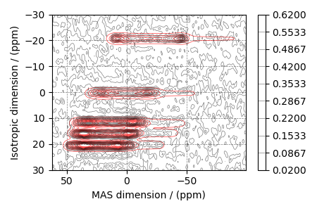
Simulate the spectrum corresponding to the optimum parameters
sim.run()
processed_data = processor.apply_operations(data=sim.methods[0].simulation).real
Plot the spectrum
ax = plt.subplot(projection="csdm")
ax.contour(processed_data, colors="r", levels=levels, alpha=0.75, linewidths=0.5)
cb = ax.contour(experiment, colors="k", levels=levels, alpha=0.5, linewidths=0.5)
plt.colorbar(cb)
ax.invert_xaxis()
ax.set_ylim(30, -30)
plt.tight_layout()
plt.show()
- 1
Grandinetti, P. J., Baltisberger, J. H., Farnan, I., Stebbins, J. F., Werner, U. and Pines, A. Solid-State \(^{17}\text{O}\) Magic-Angle and Dynamic-Angle Spinning NMR Study of the \(\text{SiO}_2\) Polymorph Coesite, J. Phys. Chem. 1995, 99, 32, 12341-12348. DOI: 10.1021/j100032a045
Total running time of the script: ( 1 minutes 50.062 seconds)