13C 2D PASS NMR of LHistidine

Coesite is a high-pressure (2-3 GPa) and high-temperature (700°C) polymorph of silicon dioxide \(\text{SiO}_2\). Coesite has five crystallographic \(^{17}\text{O}\) sites. The experimental dataset used in this example is published in Grandinetti et. al. 1

import numpy as np
import csdmpy as cp
import matplotlib as mpl
import matplotlib.pyplot as plt
import mrsimulator.signal_processing as sp
import mrsimulator.signal_processing.apodization as apo
from mrsimulator import Simulator
from mrsimulator.methods import SSB2D
from mrsimulator.utils import get_spectral_dimensions
from mrsimulator.utils.spectral_fitting import LMFIT_min_function, make_LMFIT_params
from lmfit import Minimizer, report_fit
from mrsimulator.utils.collection import single_site_system_generator

# global plot configuration
mpl.rcParams["figure.figsize"] = [4.5, 3.0]

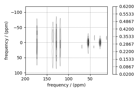
Import the dataset

filename = "https://sandbox.zenodo.org/record/687656/files/1H13C_CPPASS_LHistidine.csdf"
pass_data = cp.load(filename)

# For the spectral fitting, we only focus on the real part of the complex dataset.
# The script assumes that the dimension at index 0 is the isotropic dimension.
# Transpose the dataset as required.
pass_data = pass_data.real.T

# Convert the coordinates along each dimension from Hz to ppm.
_ = [item.to("ppm", "nmr_frequency_ratio") for item in pass_data.dimensions]

# Normalize the spectrum
pass_data /= pass_data.max()

# plot of the dataset.
levels = (np.arange(10) + 0.3) / 15  # contours are drawn at these levels.
ax = plt.subplot(projection="csdm")
cb = ax.contour(pass_data, colors="k", levels=levels, alpha=0.5, linewidths=0.5)
plt.colorbar(cb)
ax.set_xlim(200, 10)
ax.invert_yaxis()
plt.tight_layout()
plt.show()

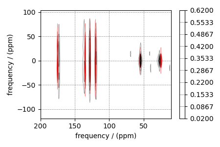
Create a fitting model

The fitting model includes the Simulator and the SignalProcessor objects. First create the Simulator object.

# Create the guess sites and spin systems.
# default unit of isotropic_chemical_shift is ppm and Cq is Hz.
shifts = [120, 128, 135, 175, 55, 25]  # in ppm
zeta = [-70, -65, -60, -60, -10, -10]  # in  Hz
eta = [0.8, 0.4, 0.9, 0.3, 0.0, 0.0]

spin_systems = single_site_system_generator(
    isotopes="13C",
    isotropic_chemical_shifts=shifts,
    shielding_symmetric={"zeta": zeta, "eta": eta},
    abundance=100 / 6,
)

# Create the DAS method.
# Get the spectral dimension paramters from the experiment.
spectral_dims = get_spectral_dimensions(pass_data)

ssb = SSB2D(
    channels=["13C"],
    magnetic_flux_density=9.4,  # in T
    rotor_frequency=1500,  # in Hz
    spectral_dimensions=spectral_dims,
    experiment=pass_data,  # also add the measurement to the method.
)

# Optimize the script by pre-setting the transition pathways for each spin system from
# the das method.
for sys in spin_systems:
    sys.transition_pathways = ssb.get_transition_pathways(sys)

# Create the Simulator object and add the method and spin system objects.
sim = Simulator()
sim.spin_systems = spin_systems  # add the spin systems
sim.methods = [ssb]  # add the method
sim.run()

# Add Post simulation processing
processor = sp.SignalProcessor(
    operations=[
        # Gaussian convolution along the isotropic dimensions.
        sp.FFT(axis=0),
        apo.Exponential(FWHM="20 Hz"),
        sp.IFFT(axis=0),
        sp.Scale(factor=0.6),
    ]
)
# Apply post simulation operations
processed_data = processor.apply_operations(data=sim.methods[0].simulation).real

# The plot of the simulation after signal processing.
ax = plt.subplot(projection="csdm")
ax.contour(processed_data, colors="r", levels=levels, alpha=0.5, linewidths=0.5)
cb = ax.contour(pass_data, colors="k", levels=levels, alpha=0.5, linewidths=0.5)
plt.colorbar(cb)
ax.set_xlim(200, 10)
plt.tight_layout()
plt.show()

Least-squares minimization with LMFIT

First create the fitting parameters. Use the make_LMFIT_params() for a quick setup.

params = make_LMFIT_params(sim, processor)
print(params.pretty_print())

Out:

Name                                      Value      Min      Max   Stderr     Vary     Expr Brute_Step
operation_1_Exponential_FWHM                 20     -inf      inf     None     True     None     None
operation_3_Scale_factor                    0.6     -inf      inf     None     True     None     None
sys_0_abundance                           16.67        0      100     None     True     None     None
sys_0_site_0_isotropic_chemical_shift       120     -inf      inf     None     True     None     None
sys_0_site_0_shielding_symmetric_eta        0.8        0        1     None     True     None     None
sys_0_site_0_shielding_symmetric_zeta       -70     -inf      inf     None     True     None     None
sys_1_abundance                           16.67        0      100     None     True     None     None
sys_1_site_0_isotropic_chemical_shift       128     -inf      inf     None     True     None     None
sys_1_site_0_shielding_symmetric_eta        0.4        0        1     None     True     None     None
sys_1_site_0_shielding_symmetric_zeta       -65     -inf      inf     None     True     None     None
sys_2_abundance                           16.67        0      100     None     True     None     None
sys_2_site_0_isotropic_chemical_shift       135     -inf      inf     None     True     None     None
sys_2_site_0_shielding_symmetric_eta        0.9        0        1     None     True     None     None
sys_2_site_0_shielding_symmetric_zeta       -60     -inf      inf     None     True     None     None
sys_3_abundance                           16.67        0      100     None     True     None     None
sys_3_site_0_isotropic_chemical_shift       175     -inf      inf     None     True     None     None
sys_3_site_0_shielding_symmetric_eta        0.3        0        1     None     True     None     None
sys_3_site_0_shielding_symmetric_zeta       -60     -inf      inf     None     True     None     None
sys_4_abundance                           16.67        0      100     None     True     None     None
sys_4_site_0_isotropic_chemical_shift        55     -inf      inf     None     True     None     None
sys_4_site_0_shielding_symmetric_eta          0        0        1     None     True     None     None
sys_4_site_0_shielding_symmetric_zeta       -10     -inf      inf     None     True     None     None
sys_5_abundance                           16.67        0      100     None    False 100-sys_0_abundance-sys_1_abundance-sys_2_abundance-sys_3_abundance-sys_4_abundance     None
sys_5_site_0_isotropic_chemical_shift        25     -inf      inf     None     True     None     None
sys_5_site_0_shielding_symmetric_eta          0        0        1     None     True     None     None
sys_5_site_0_shielding_symmetric_zeta       -10     -inf      inf     None     True     None     None
None

Run the minimization using LMFIT

minner = Minimizer(LMFIT_min_function, params, fcn_args=(sim, processor))
result = minner.minimize()
report_fit(result)

Out:

[[Fit Statistics]]
    # fitting method   = leastsq
    # function evals   = 288
    # data points      = 32768
    # variables        = 25
    chi-square         = 0.24900550
    reduced chi-square = 7.6048e-06
    Akaike info crit   = -386202.407
    Bayesian info crit = -385992.477
[[Variables]]
    sys_0_site_0_isotropic_chemical_shift:  119.106046 +/- 0.00370472 (0.00%) (init = 120)
    sys_0_site_0_shielding_symmetric_zeta: -72.0665767 +/- 0.32561995 (0.45%) (init = -70)
    sys_0_site_0_shielding_symmetric_eta:   0.98532915 +/- 0.00760810 (0.77%) (init = 0.8)
    sys_0_abundance:                        16.2131303 +/- 0.07746184 (0.48%) (init = 16.66667)
    sys_1_site_0_isotropic_chemical_shift:  128.128413 +/- 0.00311088 (0.00%) (init = 128)
    sys_1_site_0_shielding_symmetric_zeta: -75.5968193 +/- 0.27328472 (0.36%) (init = -65)
    sys_1_site_0_shielding_symmetric_eta:   0.94580299 +/- 0.00579597 (0.61%) (init = 0.4)
    sys_1_abundance:                        20.4664007 +/- 0.07798771 (0.38%) (init = 16.66667)
    sys_2_site_0_isotropic_chemical_shift:  136.122892 +/- 0.00473325 (0.00%) (init = 135)
    sys_2_site_0_shielding_symmetric_zeta: -86.2835196 +/- 0.38552276 (0.45%) (init = -60)
    sys_2_site_0_shielding_symmetric_eta:   0.42623625 +/- 0.00813561 (1.91%) (init = 0.9)
    sys_2_abundance:                        12.3406889 +/- 0.07816727 (0.63%) (init = 16.66667)
    sys_3_site_0_isotropic_chemical_shift:  172.906078 +/- 0.00306329 (0.00%) (init = 175)
    sys_3_site_0_shielding_symmetric_zeta: -69.4823878 +/- 0.25495175 (0.37%) (init = -60)
    sys_3_site_0_shielding_symmetric_eta:   0.99764477 +/- 0.00633951 (0.64%) (init = 0.3)
    sys_3_abundance:                        19.3309855 +/- 0.07589593 (0.39%) (init = 16.66667)
    sys_4_site_0_isotropic_chemical_shift:  54.4880968 +/- 0.00146751 (0.00%) (init = 55)
    sys_4_site_0_shielding_symmetric_zeta: -20.0861214 +/- 0.12734617 (0.63%) (init = -10)
    sys_4_site_0_shielding_symmetric_eta:   0.41793437 +/- 0.03977290 (9.52%) (init = 0)
    sys_4_abundance:                        18.1291926 +/- 0.05433628 (0.30%) (init = 16.66667)
    sys_5_site_0_isotropic_chemical_shift:  26.9768352 +/- 0.00161380 (0.01%) (init = 25)
    sys_5_site_0_shielding_symmetric_zeta: -10.3529547 +/- 0.53266920 (5.15%) (init = -10)
    sys_5_site_0_shielding_symmetric_eta:   0.71438965 +/- 0.24213064 (33.89%) (init = 0)
    sys_5_abundance:                        13.5196021 +/- 0.05051756 (0.37%) == '100-sys_0_abundance-sys_1_abundance-sys_2_abundance-sys_3_abundance-sys_4_abundance'
    operation_1_Exponential_FWHM:           98.6457994 +/- 0.31250846 (0.32%) (init = 20)
    operation_3_Scale_factor:               0.51492602 +/- 0.00116100 (0.23%) (init = 0.6)
[[Correlations]] (unreported correlations are < 0.100)
    C(sys_5_site_0_shielding_symmetric_zeta, sys_5_site_0_shielding_symmetric_eta) =  0.929
    C(sys_4_site_0_shielding_symmetric_zeta, sys_4_site_0_shielding_symmetric_eta) =  0.719
    C(operation_1_Exponential_FWHM, operation_3_Scale_factor)                      =  0.563
    C(sys_1_site_0_shielding_symmetric_zeta, sys_1_site_0_shielding_symmetric_eta) =  0.438
    C(sys_3_site_0_shielding_symmetric_zeta, sys_3_site_0_shielding_symmetric_eta) =  0.433
    C(sys_0_site_0_shielding_symmetric_zeta, sys_0_site_0_shielding_symmetric_eta) =  0.430
    C(sys_2_site_0_shielding_symmetric_zeta, sys_2_site_0_shielding_symmetric_eta) =  0.340
    C(sys_4_site_0_shielding_symmetric_zeta, sys_4_abundance)                      = -0.291
    C(sys_0_site_0_shielding_symmetric_zeta, sys_0_abundance)                      = -0.291
    C(sys_3_site_0_shielding_symmetric_zeta, sys_3_abundance)                      = -0.284
    C(sys_4_abundance, operation_3_Scale_factor)                               = -0.277
    C(sys_0_abundance, sys_1_abundance)                               = -0.274
    C(sys_1_site_0_shielding_symmetric_zeta, sys_1_abundance)                      = -0.270
    C(sys_1_abundance, sys_2_abundance)                               = -0.269
    C(sys_1_abundance, sys_3_abundance)                               = -0.263
    C(sys_0_abundance, sys_3_abundance)                               = -0.257
    C(sys_2_abundance, sys_3_abundance)                               = -0.247
    C(sys_0_abundance, sys_2_abundance)                               = -0.232
    C(sys_2_site_0_shielding_symmetric_eta, sys_2_abundance)                       =  0.223
    C(sys_2_site_0_shielding_symmetric_zeta, sys_2_abundance)                      = -0.218
    C(sys_2_abundance, sys_4_abundance)                               = -0.207
    C(sys_1_site_0_isotropic_chemical_shift, sys_1_abundance)                      =  0.199
    C(sys_0_abundance, sys_4_abundance)                               = -0.183
    C(sys_4_site_0_isotropic_chemical_shift, operation_1_Exponential_FWHM)         = -0.162
    C(sys_2_abundance, operation_3_Scale_factor)                               =  0.161
    C(sys_1_site_0_isotropic_chemical_shift, operation_1_Exponential_FWHM)         = -0.160
    C(sys_4_site_0_shielding_symmetric_eta, sys_4_abundance)                       =  0.157
    C(sys_3_abundance, sys_4_abundance)                               = -0.157
    C(sys_1_abundance, sys_4_abundance)                               = -0.152
    C(sys_3_site_0_shielding_symmetric_zeta, operation_3_Scale_factor)             = -0.118
    C(sys_0_site_0_shielding_symmetric_zeta, operation_3_Scale_factor)             = -0.116
    C(sys_1_site_0_shielding_symmetric_zeta, operation_3_Scale_factor)             = -0.114

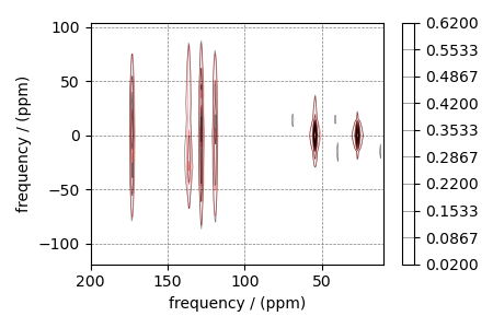
Simulate the spectrum corresponding to the optimum parameters

sim.run()
processed_data = processor.apply_operations(data=sim.methods[0].simulation).real

Plot the spectrum

ax = plt.subplot(projection="csdm")
ax.contour(processed_data, colors="r", levels=levels, alpha=0.5, linewidths=0.5)
cb = ax.contour(pass_data, colors="k", levels=levels, alpha=0.5, linewidths=0.5)
plt.colorbar(cb)
ax.set_xlim(200, 10)
plt.tight_layout()
plt.show()

1

Grandinetti, P. J., Baltisberger, J. H., Farnan, I., Stebbins, J. F., Werner, U. and Pines, A. Solid-State \(^{17}\text{O}\) Magic-Angle and Dynamic-Angle Spinning NMR Study of the \(\text{SiO}_2\) Polymorph Coesite, J. Phys. Chem. 1995, 99, 32, 12341-12348. DOI: 10.1021/j100032a045