Selective Excitations using Custom Isotopes

Simulating spectra of custom isotopes

The isotope register method has the copy_from argument which can be used to create individually addressable channels which the same isotope attributes. This functionality can be used to emulate selective-excitation experiments by querying specific transitions on different sites

from mrsimulator.spin_system.isotope import Isotope
from mrsimulator import Site, SpinSystem, Coupling, Simulator, Method
from mrsimulator.method import SpectralDimension, SpectralEvent
from mrsimulator.method.lib import BlochDecaySpectrum
from mrsimulator.method.query import TransitionQuery
import mrsimulator.signal_processor as sp

from pprint import pprint
import matplotlib.pyplot as plt

Below, we show how custom isotopes can be copied from existing isotopes, and how these custom isotopes can be used to simulate a selective-excitation spectrum of protons. First, two new isotopes – "1H-a" and "1H-b" – are registered from the known proton isotope by using the copy_from keyword argument.

Isotope.register("1H-a", copy_from="1H")
Isotope.register("1H-b", copy_from="1H")

Next, we create two site objects using the previously registered "1H-a" and "1H-b" isotope symbols. The equivalent proton system (without custom isotopes) is also constructed as a comparison.

site_a = Site(isotope="1H", isotropic_chemical_shift=-0.5)
site_b = Site(isotope="1H", isotropic_chemical_shift=-2.0)
coupling_ab = Coupling(site_index=[0, 1], isotropic_j=48)
sys = SpinSystem(sites=[site_a, site_b], couplings=[coupling_ab])  # proton system

# Create 1D BlochDecaySpectrum for proton
spec_dim = SpectralDimension(count=10000, spectral_width=2000, reference_offset=-500)
mth = BlochDecaySpectrum(channels=["1H"], spectral_dimensions=[spec_dim])

# Create Simulator object for coupled proton system
sim = Simulator(spin_systems=[sys], methods=[mth])


# Create couple proton system from custom isotopes
site_a_custom = Site(isotope="1H-a", isotropic_chemical_shift=-0.5)
site_b_custom = Site(isotope="1H-b", isotropic_chemical_shift=-2.0)
sys_custom = SpinSystem(sites=[site_a_custom, site_b_custom], couplings=[coupling_ab])

# Create two BlochDecaySpectrum methods with custom isotope channels
mth_a = BlochDecaySpectrum(channels=["1H-a"], spectral_dimensions=[spec_dim])
mth_b = BlochDecaySpectrum(channels=["1H-b"], spectral_dimensions=[spec_dim])

Create and run two simulator objects for the simulating the regular and selective excitation proton spectra.

sim = Simulator(spin_systems=[sys], methods=[mth])
sim_custom = Simulator(spin_systems=[sys_custom], methods=[mth_a, mth_b])

# Run both the simulations
sim.run()
sim_custom.run()

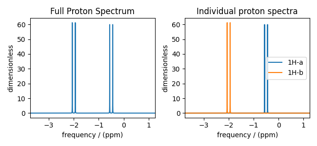
Apply post-simulation signal processing and plot the spectra. Notice how the full proton spectrum (right) is the summation of the two individual proton spectra (left), and how the J-couplings are still present in the selective excitation spectra. Make processor for adding line broadening to spectra

processor = sp.SignalProcessor(
    operations=[sp.FFT(), sp.apodization.Exponential(FWHM="1 Hz"), sp.IFFT()]
)
spec_proton = processor.apply_operations(sim.methods[0].simulation).real
spec_a = processor.apply_operations(sim_custom.methods[0].simulation).real
spec_b = processor.apply_operations(sim_custom.methods[1].simulation).real

fig, ax = plt.subplots(1, 2, figsize=(6.5, 3), subplot_kw={"projection": "csdm"})

ax[0].plot(spec_proton)
ax[0].set_title("Full Proton Spectrum")
ax[1].plot(spec_a, label="1H-a")
ax[1].plot(spec_b, label="1H-b")
ax[1].legend()
ax[1].set_title("Individual proton spectra")

plt.tight_layout()
plt.show()

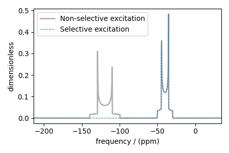
Custom isotopes can be used in conjunction with custom method objects to query different transitions on custom isotopes. Below, we create a custom Method which simulates a coupled 1H-13C spectrum where the carbon site simultaneous undergoes a transitions with only one of the proton sites.

proton_a_custom = Site(isotope="1H-a", isotropic_chemical_shift=0.0)
proton_b_custom = Site(isotope="1H-b", isotropic_chemical_shift=20)
carbon = Site(isotope="13C", isotropic_chemical_shift=-40)

# J- and dipolar-couplings for the system
coupling_ab = Coupling(site_index=[0, 1], isotropic_j=48)  # 1H-a, 1H-b
coupling_ac = Coupling(site_index=[0, 2], dipolar={"D": 2000})  # 1H-a, 13C
coupling_bc = Coupling(site_index=[1, 2], dipolar={"D": 1000})  # 1H-b, 13C

sys_custom = SpinSystem(
    sites=[proton_a_custom, proton_b_custom, carbon],
    couplings=[coupling_ab, coupling_ac, coupling_bc],
)

Next, we create the Method object which has three different channels; the first channel is the observed nucleus, here 13C, and the other two are for the custom proton isotopes.

mth_custom = Method(
    channels=["13C", "1H-a", "1H-b"],
    spectral_dimensions=[
        SpectralDimension(
            reference_offset=-9000,
            events=[
                SpectralEvent(
                    transition_queries=[
                        TransitionQuery(
                            ch1={"P": [-1]}, ch2={"P": [-1]}, ch3={"P": [0]}
                        )
                    ]
                )
            ],
        )
    ],
)
pprint(mth_custom.get_transition_pathways(sys_custom))

[|-0.5, -0.5, -0.5⟩⟨0.5, -0.5, 0.5|, weight=(1+0j),
 |-0.5, 0.5, -0.5⟩⟨0.5, 0.5, 0.5|, weight=(1+0j)]

The equivalent SpinSystem and Method without custom isotopes or selective excitations as a comparison.

proton_a = Site(isotope="1H", isotropic_chemical_shift=0.0)
proton_b = Site(isotope="1H", isotropic_chemical_shift=-20)
carbon = Site(isotope="13C", isotropic_chemical_shift=-40)

# J- and dipolar-couplings for the system
coupling_ab = Coupling(site_index=[0, 1], isotropic_j=48)  # 1H-a, 1H-b
coupling_ac = Coupling(site_index=[0, 2], dipolar={"D": 2000})  # 1H-a, 13C
coupling_bc = Coupling(site_index=[1, 2], dipolar={"D": 1000})  # 1H-b, 13C

sys = SpinSystem(
    sites=[proton_a, proton_b, carbon],
    couplings=[coupling_ab, coupling_ac, coupling_bc],
)

mth = Method(
    channels=["13C", "1H"],
    spectral_dimensions=[
        SpectralDimension(
            reference_offset=-9000,
            events=[
                SpectralEvent(
                    transition_queries=[
                        TransitionQuery(
                            ch1={"P": [-1]},
                            ch2={"P": [-1]},
                        )
                    ]
                )
            ],
        )
    ],
)
pprint(mth.get_transition_pathways(sys))

[|-0.5, -0.5, -0.5⟩⟨-0.5, 0.5, 0.5|, weight=(1+0j),
 |-0.5, -0.5, -0.5⟩⟨0.5, -0.5, 0.5|, weight=(1+0j),
 |-0.5, 0.5, -0.5⟩⟨0.5, 0.5, 0.5|, weight=(1+0j),
 |0.5, -0.5, -0.5⟩⟨0.5, 0.5, 0.5|, weight=(1+0j)]

Create and run Simulator objects for the selective and non-selective spectra.

sim_custom = Simulator(spin_systems=[sys_custom], methods=[mth_custom])
sim = Simulator(spin_systems=[sys], methods=[mth])

sim_custom.run()
sim.run()

Plot the simulated spectra

plt.figure(figsize=(4.5, 3))
plt.subplot(projection="csdm")
plt.plot(
    sim.methods[0].simulation.real,
    color="black",
    alpha=0.3,
    linewidth=2,
    label="Non-selective excitation",
)
plt.plot(
    sim_custom.methods[0].simulation.real,
    linestyle="--",
    alpha=1.0,
    linewidth=0.75,
    label="Selective excitation",
)

plt.legend()
plt.tight_layout()
plt.show()