Note
Go to the end to download the full example code.
Potassium Sulfate, ³³S (I=3/2)
³³S (I=3/2) quadrupolar spectrum simulation.
The following example is the \(^{33}\text{S}\) NMR spectrum simulation of potassium sulfate (\(\text{K}_2\text{SO}_4\)). The quadrupole tensor parameters for \(^{33}\text{S}\) is obtained from Moudrakovski et al. [1]
import matplotlib.pyplot as plt

from mrsimulator import Simulator, SpinSystem, Site
from mrsimulator import signal_processor as sp
from mrsimulator.method.lib import BlochDecayCTSpectrum
from mrsimulator.spin_system.tensors import SymmetricTensor
from mrsimulator.method import SpectralDimension
Create the spin system
site = Site(
    name="33S",
    isotope="33S",
    isotropic_chemical_shift=335.7,  # in ppm
    quadrupolar=SymmetricTensor(Cq=0.959e6, eta=0.42),  # Cq is in Hz
)
spin_system = SpinSystem(sites=[site])
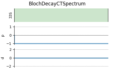
Create a central transition selective Bloch decay spectrum method.
method = BlochDecayCTSpectrum(
    channels=["33S"],
    magnetic_flux_density=21.14,  # in T
    rotor_frequency=14000,  # in Hz
    spectral_dimensions=[
        SpectralDimension(
            count=2048,
            spectral_width=5000,  # in Hz
            reference_offset=22500,  # in Hz
            label=r"$^{33}$S resonances",
        )
    ],
)

# A graphical representation of the method object.
plt.figure(figsize=(4, 2.5))
method.plot()
plt.show()
Create the Simulator object and add method and spin system objects.
sim = Simulator(spin_systems=[spin_system], methods=[method])
sim.run()
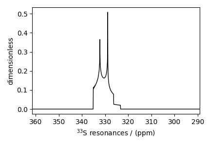
# The plot of the simulation before signal processing.
plt.figure(figsize=(4.25, 3.0))
ax = plt.subplot(projection="csdm")
ax.plot(sim.methods[0].simulation.real, color="black", linewidth=1)
ax.invert_xaxis()
plt.tight_layout()
plt.show()
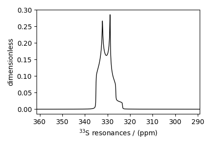
Add post-simulation signal processing.
processor = sp.SignalProcessor(
    operations=[sp.IFFT(), sp.apodization.Exponential(FWHM="10 Hz"), sp.FFT()]
)
processed_dataset = processor.apply_operations(dataset=sim.methods[0].simulation)

# The plot of the simulation after signal processing.
plt.figure(figsize=(4.25, 3.0))
ax = plt.subplot(projection="csdm")
ax.plot(processed_dataset.real, color="black", linewidth=1)
ax.invert_xaxis()
plt.tight_layout()
plt.show()
Total running time of the script: (0 minutes 0.384 seconds)