Note
Go to the end to download the full example code.
Coesite, ¹⁷O (I=5/2)
¹⁷O (I=5/2) quadrupolar spectrum simulation.
Coesite is a high-pressure (2-3 GPa) and high-temperature (700°C) polymorph of silicon dioxide \(\text{SiO}_2\). Coesite has five crystallographic \(^{17}\text{O}\) sites. In the following, we use the \(^{17}\text{O}\) EFG tensor information from Grandinetti et al. [1]
import matplotlib.pyplot as plt

from mrsimulator import Simulator, SpinSystem, Site
from mrsimulator import signal_processor as sp
from mrsimulator.method.lib import BlochDecayCTSpectrum
from mrsimulator.spin_system.tensors import SymmetricTensor
from mrsimulator.method import SpectralDimension
Create the sites.
# default unit of isotropic_chemical_shift is ppm and Cq is Hz.
O17_1 = Site(
    isotope="17O",
    isotropic_chemical_shift=29,
    quadrupolar=SymmetricTensor(Cq=6.05e6, eta=0.000),
)
O17_2 = Site(
    isotope="17O",
    isotropic_chemical_shift=41,
    quadrupolar=SymmetricTensor(Cq=5.43e6, eta=0.166),
)
O17_3 = Site(
    isotope="17O",
    isotropic_chemical_shift=57,
    quadrupolar=SymmetricTensor(Cq=5.45e6, eta=0.168),
)
O17_4 = Site(
    isotope="17O",
    isotropic_chemical_shift=53,
    quadrupolar=SymmetricTensor(Cq=5.52e6, eta=0.169),
)
O17_5 = Site(
    isotope="17O",
    isotropic_chemical_shift=58,
    quadrupolar=SymmetricTensor(Cq=5.16e6, eta=0.292),
)

# all five sites.
sites = [O17_1, O17_2, O17_3, O17_4, O17_5]
Create the spin systems from these sites. For optimum performance, we create five single-site spin systems instead of a single five-site spin system. The abundance of each spin system is taken from above reference. Here we are iterating over both the sites and abundance list concurrently using a list comprehension to construct a list of SpinSystems
abundance = [0.83, 1.05, 2.16, 2.05, 1.90]
spin_systems = [SpinSystem(sites=[s], abundance=a) for s, a in zip(sites, abundance)]
Create a central transition selective Bloch decay spectrum method.
method = BlochDecayCTSpectrum(
    channels=["17O"],
    rotor_frequency=14000,  # in Hz
    spectral_dimensions=[
        SpectralDimension(
            count=2048,
            spectral_width=50000,  # in Hz
            label=r"$^{17}$O resonances",
        )
    ],
)
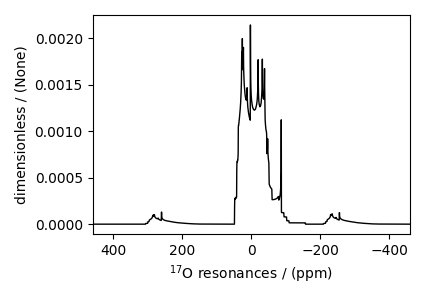
The above method is set up to record the \(^{17}\text{O}\) resonances at the magic angle, spinning at 14 kHz and 9.4 T (default, if the value is not provided) external magnetic flux density. The resonances are recorded over 50 kHz spectral width using 2048 points.
Create the Simulator object and add method and spin system objects.
sim = Simulator(spin_systems=spin_systems, methods=[method])
sim.run()

# The plot of the simulation before signal processing.
plt.figure(figsize=(4.25, 3.0))
ax = plt.subplot(projection="csdm")
ax.plot(sim.methods[0].simulation.real, color="black", linewidth=1)
ax.invert_xaxis()
plt.tight_layout()
plt.show()
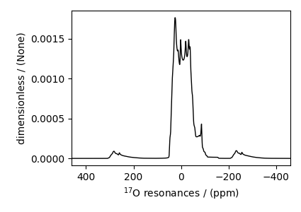
Add post-simulation signal processing.
processor = sp.SignalProcessor(
    operations=[
        sp.IFFT(),
        sp.apodization.Exponential(FWHM="30 Hz"),
        sp.apodization.Gaussian(FWHM="145 Hz"),
        sp.FFT(),
    ]
)
processed_dataset = processor.apply_operations(dataset=sim.methods[0].simulation)

# The plot of the simulation after signal processing.
plt.figure(figsize=(4.25, 3.0))
ax = plt.subplot(projection="csdm")
ax.plot(processed_dataset.real, color="black", linewidth=1)
ax.invert_xaxis()
plt.tight_layout()
plt.show()
Total running time of the script: (0 minutes 0.285 seconds)