Arbitrary spin transition (single-quantum)

²⁷Al (I=5/2) quadrupolar spectrum simulation.

The mrsimulator built-in library methods, BlochDecaySpectrum and BlochDecayCTSpectrum, simulate spectrum from single quantum transitions or central transition selective transition, respectively. In this example, we show how you can simulate any arbitrary transition using the generic Method object.

import numpy as np
import matplotlib.pyplot as plt

from mrsimulator import Simulator, SpinSystem, Site
from mrsimulator.method import Method, SpectralDimension, SpectralEvent
from mrsimulator.spin_system.tensors import SymmetricTensor

Create a single-site arbitrary spin system.

site = Site(
    name="27Al",
    isotope="27Al",
    isotropic_chemical_shift=35.7,  # in ppm
    quadrupolar=SymmetricTensor(Cq=5.959e6, eta=0.32),  # Cq is in Hz
)
spin_system = SpinSystem(sites=[site])

Selecting spin transitions for simulation

The arguments of the Method object are the same as the arguments of the BlochDecaySpectrum method; however, unlike a BlochDecaySpectrum method, the SpectralDimension object in Method contains an additional argument—events.

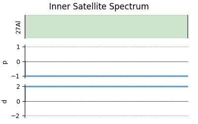
The Events object is a collection of attributes, which are local to the event. It is here where we define transition_queries to select one or more transitions for simulating the spectrum. Recall, a TransitionQuery object holds a channel wise SymmetryQuery. For more information, refer to the Spin Transition Symmetry Functions. In this example, we use the P=-1 and D=2 attributes of SymmetryQuery, to select the satellite transition, \(|-1/2\rangle\rightarrow|-3/2\rangle\).

method = Method(
    name="Inner Satellite Spectrum",
    channels=["27Al"],
    magnetic_flux_density=21.14,  # in T
    rotor_frequency=np.inf,  # in Hz
    rotor_angle=54.7356 * np.pi / 180,  # in rads
    spectral_dimensions=[
        SpectralDimension(
            count=1024,
            spectral_width=1e4,  # in Hz
            reference_offset=1e4,  # in Hz
            events=[
                SpectralEvent(
                    transition_queries=[
                        {"ch1": {"P": [-1], "D": [2]}},  # inner satellite
                    ]
                )
            ],
        )
    ],
)

# A graphical representation of the method object.
plt.figure(figsize=(4, 2.5))
method.plot()
plt.show()

Create the Simulator object and add the method and the spin system object.

sim = Simulator(spin_systems=[spin_system], methods=[method])
sim.run()

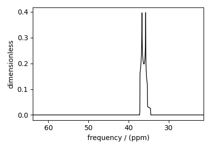
# The plot of the simulation before signal processing.
plt.figure(figsize=(4.25, 3.0))
ax = plt.subplot(projection="csdm")
ax.plot(sim.methods[0].simulation.real, color="black", linewidth=1)
ax.invert_xaxis()
plt.tight_layout()
plt.show()

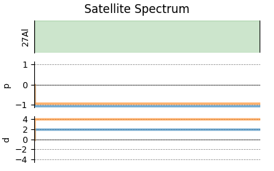
Selecting both inner and outer-satellite transitions

Similarly, you may add another transition query to select to select additional transitions. Consider the following transitions with respective P and D values.

• \(|-1/2\rangle\rightarrow|-3/2\rangle ~~ (P=-1, D=2)\)

• \(|-3/2\rangle\rightarrow|-5/2\rangle ~~ (P=-1, D=4)\)

method2 = Method(
    name="Satellite Spectrum",
    channels=["27Al"],
    magnetic_flux_density=21.14,  # in T
    rotor_frequency=np.inf,  # in Hz
    rotor_angle=54.7356 * np.pi / 180,  # in rads
    spectral_dimensions=[
        SpectralDimension(
            count=1024,
            spectral_width=1e4,  # in Hz
            reference_offset=1e4,  # in Hz
            events=[
                SpectralEvent(
                    transition_queries=[
                        {"ch1": {"P": [-1], "D": [2]}},  # inter satellite
                        {"ch1": {"P": [-1], "D": [4]}},  # outer satellite
                    ]
                )
            ],
        )
    ],
)

# A graphical representation of the method object.
plt.figure(figsize=(4, 2.5))
method2.plot()
plt.show()

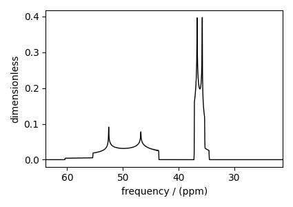
Update the method object in the Simulator object and re-simulate

sim.methods[0] = method2
sim.run()

# The plot of the simulation before signal processing.
plt.figure(figsize=(4.25, 3.0))
ax = plt.subplot(projection="csdm")
ax.plot(sim.methods[0].simulation.real, color="black", linewidth=1)
ax.invert_xaxis()
plt.tight_layout()
plt.show()