Arbitrary spin transition (multi-quantum)

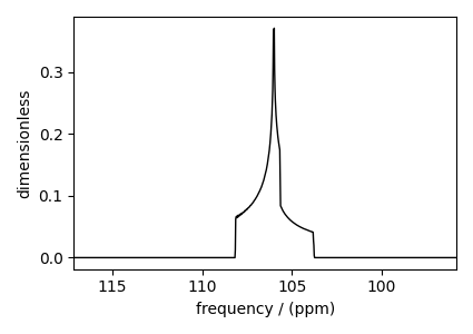
³³S (I=5/2) quadrupolar spectrum simulation.

Simulate a triple quantum spectrum.

import numpy as np
import matplotlib.pyplot as plt

from mrsimulator import Simulator, SpinSystem, Site
from mrsimulator.method import Method, SpectralDimension, SpectralEvent
from mrsimulator.spin_system.tensors import SymmetricTensor

Create a single-site arbitrary spin system.

site = Site(
    name="27Al",
    isotope="27Al",
    isotropic_chemical_shift=35.7,  # in ppm
    quadrupolar=SymmetricTensor(Cq=2.959e6, eta=0.98),  # Cq is in Hz
)
spin_system = SpinSystem(sites=[site])

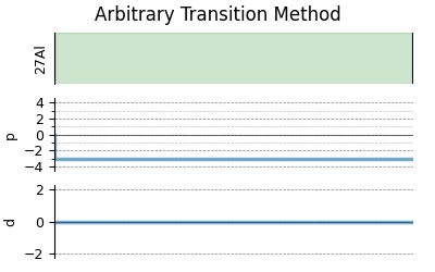
Selecting the triple-quantum transition

For single-site spin-5/2 spin system, there are three triple-quantum transition

• \(|1/2\rangle\rightarrow|-5/2\rangle\) (\(P=-3, D=6\))

• \(|3/2\rangle\rightarrow|-3/2\rangle\) (\(P=-3, D=0\))

• \(|5/2\rangle\rightarrow|-1/2\rangle\) (\(P=-3, D=-6\))

To select one or more triple-quantum transitions, assign the respective value of P and D to the symmetry query object of transition_queries. Refer to the Spin Transition Symmetry Functions for details.

Here, we select the symmetric triple-quantum transition.

method = Method(
    name="Arbitrary Transition Method",
    channels=["27Al"],
    magnetic_flux_density=21.14,  # in T
    rotor_frequency=np.inf,  # in Hz
    rotor_angle=54.7356 * np.pi / 180,  # in rads
    spectral_dimensions=[
        SpectralDimension(
            count=1024,
            spectral_width=5e3,  # in Hz
            reference_offset=2.5e4,  # in Hz
            events=[
                SpectralEvent(
                    # symmetric triple quantum transitions
                    transition_queries=[{"ch1": {"P": [-3], "D": [0]}}]
                ),
            ],
        )
    ],
)

# A graphical representation of the method object.
plt.figure(figsize=(4, 2.5))
method.plot()
plt.show()

Create the Simulator object and add the method and the spin system object.

sim = Simulator(spin_systems=[spin_system], methods=[method])
sim.run()

# The plot of the simulation before signal processing.
plt.figure(figsize=(4.25, 3.0))
ax = plt.subplot(projection="csdm")
ax.plot(sim.methods[0].simulation.real, color="black", linewidth=1)
ax.invert_xaxis()
plt.tight_layout()
plt.show()