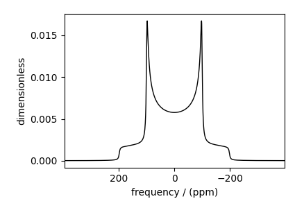
Coupled spin-1/2 (Static dipolar spectrum)

¹³C-¹H static dipolar coupling simulation.

import matplotlib.pyplot as plt

from mrsimulator import Simulator, SpinSystem, Site, Coupling
from mrsimulator.method.lib import BlochDecaySpectrum
from mrsimulator import signal_processor as sp
from mrsimulator.spin_system.tensors import SymmetricTensor
from mrsimulator.method import SpectralDimension

Create a 13C-1H coupled spin system.

spin_system = SpinSystem(
    sites=[
        Site(isotope="13C", isotropic_chemical_shift=0.0),
        Site(isotope="1H", isotropic_chemical_shift=0.0),
    ],
    couplings=[Coupling(site_index=[0, 1], dipolar=SymmetricTensor(D=-2e4))],
)

Create a BlochDecaySpectrum method.

method = BlochDecaySpectrum(
    channels=["13C"],
    magnetic_flux_density=9.4,  # in T
    rotor_frequency=0,  # in Hz
    rotor_angle=0,  # in rads
    spectral_dimensions=[SpectralDimension(count=2048, spectral_width=8.0e4)],
)

Create the Simulator object and add the method and the spin system object.

sim = Simulator(spin_systems=[spin_system], methods=[method])
sim.run()

Add post-simulation signal processing.

processor = sp.SignalProcessor(
    operations=[
        sp.IFFT(),
        sp.apodization.Exponential(FWHM="500 Hz"),
        sp.FFT(),
    ]
)
processed_dataset = processor.apply_operations(dataset=sim.methods[0].simulation)

plt.figure(figsize=(4.25, 3.0))
ax = plt.subplot(projection="csdm")
ax.plot(processed_dataset.real, color="black", linewidth=1)
ax.invert_xaxis()
plt.tight_layout()
plt.show()