Note
Go to the end to download the full example code.
RbNO₃, ⁸⁷Rb (I=3/2) STMAS
⁸⁷Rb (I=3/2) satellite-transition off magic-angle spinning simulation.
The following is an example of the STMAS simulation of \(\text{RbNO}_3\). The \(^{87}\text{Rb}\) tensor parameters were obtained from Massiot et al. [1].
import matplotlib.pyplot as plt

from mrsimulator import Simulator, SpinSystem, Site
from mrsimulator.method.lib import ST1_VAS
from mrsimulator import signal_processor as sp
from mrsimulator.spin_system.tensors import SymmetricTensor
from mrsimulator.method import SpectralDimension
Generate the site and spin system objects.
Rb87_1 = Site(
    isotope="87Rb",
    isotropic_chemical_shift=-27.4,  # in ppm
    quadrupolar=SymmetricTensor(Cq=1.68e6, eta=0.2),  # Cq is in Hz
)
Rb87_2 = Site(
    isotope="87Rb",
    isotropic_chemical_shift=-28.5,  # in ppm
    quadrupolar=SymmetricTensor(Cq=1.94e6, eta=1.0),  # Cq is in Hz
)
Rb87_3 = Site(
    isotope="87Rb",
    isotropic_chemical_shift=-31.3,  # in ppm
    quadrupolar=SymmetricTensor(Cq=1.72e6, eta=0.5),  # Cq is in Hz
)

sites = [Rb87_1, Rb87_2, Rb87_3]  # all sites
spin_systems = [SpinSystem(sites=[s]) for s in sites]
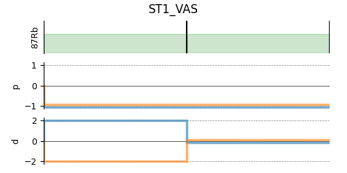
Select a satellite-transition variable-angle spinning method. The following ST1_VAS method correlates the frequencies from the two inner-satellite transitions to the central transition. Note, STMAS measurements are highly suspectable to rotor angle mismatch. In the following, we show two methods, the first at the magic angle and second deliberately miss-sets by approximately 0.0059 degrees.
angles = [54.7359, 54.73]
method = []
for angle in angles:
    method.append(
        ST1_VAS(
            channels=["87Rb"],
            magnetic_flux_density=7,  # in T
            rotor_angle=angle * 3.14159 / 180,  # in rad (magic angle)
            spectral_dimensions=[
                SpectralDimension(
                    count=256,
                    spectral_width=3e3,  # in Hz
                    reference_offset=-2.4e3,  # in Hz
                    label="Isotropic dimension",
                ),
                SpectralDimension(
                    count=512,
                    spectral_width=5e3,  # in Hz
                    reference_offset=-4e3,  # in Hz
                    label="MAS dimension",
                ),
            ],
        )
    )

# A graphical representation of the method object.
plt.figure(figsize=(5, 2.5))
method[0].plot()
plt.show()
Create the Simulator object, add the method and spin system objects, and run the simulation.
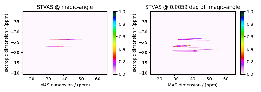
The plot of the simulation.
dataset = [sim.methods[0].simulation, sim.methods[1].simulation]
fig, ax = plt.subplots(1, 2, figsize=(8.5, 3), subplot_kw={"projection": "csdm"})

titles = ["STVAS @ magic-angle", "STVAS @ 0.0059 deg off magic-angle"]
for i, item in enumerate(dataset):
    cb1 = ax[i].imshow(item.real / item.real.max(), aspect="auto", cmap="gist_ncar_r")
    ax[i].set_title(titles[i])
    plt.colorbar(cb1, ax=ax[i])
    ax[i].invert_xaxis()
    ax[i].invert_yaxis()
plt.tight_layout()
plt.show()
Add post-simulation signal processing.
processor = sp.SignalProcessor(
    operations=[
        # Gaussian convolution along both dimensions.
        sp.IFFT(dim_index=(0, 1)),
        sp.apodization.Gaussian(FWHM="50 Hz", dim_index=0),
        sp.apodization.Gaussian(FWHM="50 Hz", dim_index=1),
        sp.FFT(dim_index=(0, 1)),
    ]
)
processed_dataset = []
for item in dataset:
    processed_dataset.append(processor.apply_operations(dataset=item))
    processed_dataset[-1] /= processed_dataset[-1].max()
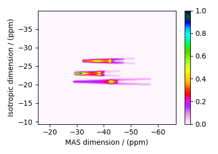
The plot of the simulation after signal processing.
plt.figure(figsize=(4.25, 3.0))
ax = plt.subplot(projection="csdm")
cb = ax.imshow(processed_dataset[1].real, cmap="gist_ncar_r", aspect="auto")
plt.colorbar(cb)
ax.invert_xaxis()
ax.invert_yaxis()
plt.tight_layout()
plt.show()
Total running time of the script: (0 minutes 0.796 seconds)