Rb₂SO₄, ⁸⁷Rb (I=3/2) SAS¶

⁸⁷Rb (I=3/2) Switched-angle spinning (SAS) simulation.

The following is an example of Switched-Angle Spinning (SAS) simulation of \(\text{Rb}_2\text{SO}_4\), which has two distinct rubidium sites. The NMR tensor parameters for these sites are taken from Shore et al. [1].

import numpy as np
import matplotlib.pyplot as plt

from mrsimulator import Simulator, SpinSystem, Site
from mrsimulator.method import Method, SpectralDimension, SpectralEvent
from mrsimulator import signal_processor as sp
from mrsimulator.spin_system.tensors import SymmetricTensor

Generate the site and spin system objects.

sites = [
    Site(
        isotope="87Rb",
        isotropic_chemical_shift=16,  # in ppm
        quadrupolar=SymmetricTensor(Cq=5.3e6, eta=0.1),  # Cq in Hz
    ),
    Site(
        isotope="87Rb",
        isotropic_chemical_shift=40,  # in ppm
        quadrupolar=SymmetricTensor(Cq=2.6e6, eta=1.0),  # Cq in Hz
    ),
]
spin_systems = [SpinSystem(sites=[s]) for s in sites]

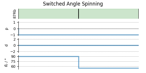
Use the generic Method class to simulate a 2D SAS spectrum by customizing the method parameters, as shown below.

sas = Method(
    name="Switched Angle Spinning",
    channels=["87Rb"],
    magnetic_flux_density=9.4,  # in T
    rotor_frequency=np.inf,
    spectral_dimensions=[
        SpectralDimension(
            count=256,
            spectral_width=3.5e4,  # in Hz
            reference_offset=1e3,  # in Hz
            label="90 dimension",
            events=[
                SpectralEvent(
                    rotor_angle=90 * np.pi / 180,  # in radians
                    transition_queries=[{"ch1": {"P": [-1], "D": [0]}}],
                )
            ],
        ),
        SpectralDimension(
            count=256,
            spectral_width=22e3,  # in Hz
            reference_offset=-4e3,  # in Hz
            label="MAS dimension",
            events=[
                SpectralEvent(
                    rotor_angle=54.74 * np.pi / 180,  # in radians
                    transition_queries=[{"ch1": {"P": [-1], "D": [0]}}],
                )
            ],
        ),
    ],
)

# A graphical representation of the method object.
plt.figure(figsize=(5, 2.5))
sas.plot()
plt.show()

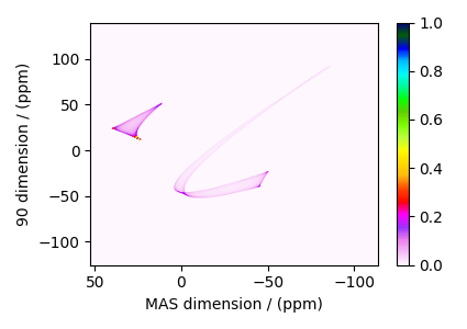
Create the Simulator object, add the method and spin system objects, and run the simulation.

sim = Simulator(spin_systems=spin_systems, methods=[sas])
sim.run()

The plot of the simulation.

dataset = sim.methods[0].simulation

plt.figure(figsize=(4.25, 3.0))
ax = plt.subplot(projection="csdm")
cb = ax.imshow(dataset.real / dataset.real.max(), aspect="auto", cmap="gist_ncar_r")
plt.colorbar(cb)
ax.invert_xaxis()
plt.tight_layout()
plt.show()

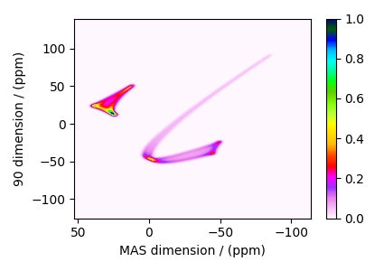
Add post-simulation signal processing.

processor = sp.SignalProcessor(
    operations=[
        # Gaussian convolution along both dimensions.
        sp.IFFT(dim_index=(0, 1)),
        sp.apodization.Gaussian(FWHM="0.4 kHz", dim_index=0),
        sp.apodization.Gaussian(FWHM="0.4 kHz", dim_index=1),
        sp.FFT(dim_index=(0, 1)),
    ]
)
processed_dataset = processor.apply_operations(dataset=dataset)
processed_dataset /= processed_dataset.max()

The plot of the simulation after signal processing.

plt.figure(figsize=(4.25, 3.0))
ax = plt.subplot(projection="csdm")
cb = ax.imshow(processed_dataset.real, cmap="gist_ncar_r", aspect="auto")
plt.colorbar(cb)
ax.invert_xaxis()
plt.tight_layout()
plt.show()

Total running time of the script: (0 minutes 1.100 seconds)

Gallery generated by Sphinx-Gallery