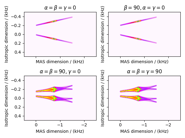
Co59 (I=7/2) STMAS

Co59 (I=7/2) satellite-transition magic-angle spinning simulation. (Quad-csa cross terms)

import numpy as np
import matplotlib.pyplot as plt

from mrsimulator import Simulator, SpinSystem, Site
from mrsimulator.method.lib import ST1_VAS
from mrsimulator import signal_processor as sp
from mrsimulator.spin_system.tensors import SymmetricTensor
from mrsimulator.method import SpectralDimension

Generate the site and spin system objects.

Co_sites = [
    Site(
        isotope="59Co",  # 59Co
        isotropic_chemical_shift=0,  # in ppm
        shielding_symmetric=SymmetricTensor(zeta=-1750, eta=1),
        quadrupolar=SymmetricTensor(Cq=3.1e6, eta=1),  # Cq is in Hz
        name="$\\alpha=\\beta=\\gamma=0$",
    ),
    Site(
        isotope="59Co",  # 59Co
        isotropic_chemical_shift=0,  # in ppm
        shielding_symmetric=SymmetricTensor(zeta=-1750, eta=1),
        quadrupolar=SymmetricTensor(Cq=3.1e6, eta=1, beta=np.pi / 2),  # Cq is in Hz
        name="$\\beta=90, \\alpha=\\gamma=0$",
    ),
    Site(
        isotope="59Co",  # 59Co
        isotropic_chemical_shift=0,  # in ppm
        shielding_symmetric=SymmetricTensor(zeta=-1750, eta=1),
        quadrupolar=SymmetricTensor(
            Cq=3.1e6, eta=1, alpha=np.pi / 2, beta=np.pi / 2
        ),  # Cq is in Hz
        name="$\\alpha=\\beta=90, \\gamma=0$",
    ),
    Site(
        isotope="59Co",  # 59Co
        isotropic_chemical_shift=0,  # in ppm
        shielding_symmetric=SymmetricTensor(zeta=-1750, eta=1),
        quadrupolar=SymmetricTensor(
            Cq=3.1e6, eta=1, alpha=np.pi / 2, beta=np.pi / 2, gamma=np.pi / 2
        ),  # Cq is in Hz
        name="$\\alpha=\\beta=\\gamma=90$",
    ),
]

spin_systems = [SpinSystem(sites=[site], name=site.name) for site in Co_sites]

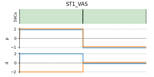
Select a satellite-transition variable-angle spinning method. The following ST1_VAS method correlates the frequencies from the two inner-satellite transitions to the central transition.

method = ST1_VAS(
    channels=["59Co"],
    magnetic_flux_density=4.684,  # in T
    rotor_angle=54.7359 * 3.14159 / 180,  # in rad (magic angle)
    spectral_dimensions=[
        SpectralDimension(
            count=256,
            spectral_width=1e3,  # in Hz
            label="Isotropic dimension",
        ),
        SpectralDimension(
            count=512,
            spectral_width=3e3,  # in Hz
            reference_offset=-1e3,  # in Hz
            label="MAS dimension",
        ),
    ],
)

# A graphical representation of the method object.
plt.figure(figsize=(5, 2.5))
method.plot()
plt.show()

Create the Simulator object, add the method and spin system objects, and run the simulation.

sim = Simulator(spin_systems=spin_systems, methods=[method])
sim.config.decompose_spectrum = "spin_system"
sim.run()

Add post-simulation signal processing.

dataset = sim.methods[0].simulation
processor = sp.SignalProcessor(
    operations=[
        # Gaussian convolution along both dimensions.
        sp.IFFT(dim_index=(0, 1)),
        sp.apodization.Gaussian(FWHM="20 Hz", dim_index=0),
        sp.apodization.Gaussian(FWHM="20 Hz", dim_index=1),
        sp.FFT(dim_index=(0, 1)),
    ]
)

processed_dataset = processor.apply_operations(dataset=dataset)

The plot of the simulation.

_ = [item.to("kHz", "nmr_frequency_ratio") for item in processed_dataset.x]

processed_dataset = processed_dataset.split()
fig, ax = plt.subplots(
    2, 2, figsize=(6, 4.5), sharex=True, sharey=True, subplot_kw={"projection": "csdm"}
)
ax[0, 0].imshow(processed_dataset[0].real, cmap="gist_ncar_r", aspect="auto")
ax[0, 1].imshow(processed_dataset[1].real, cmap="gist_ncar_r", aspect="auto")
ax[1, 0].imshow(processed_dataset[2].real, cmap="gist_ncar_r", aspect="auto")
ax[1, 1].imshow(processed_dataset[3].real, cmap="gist_ncar_r", aspect="auto")
ax[0, 0].invert_xaxis()
ax[0, 0].invert_yaxis()
plt.tight_layout()
plt.show()