Rb₂SO₄, ⁸⁷Rb (I=3/2) QMAT

⁸⁷Rb (I=3/2) Quadrupolar Magic-angle turning (QMAT) simulation.

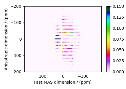
The following is a simulation of the QMAT spectrum of \(\text{Rb}_2\text{SiO}_4\). The 2D QMAT spectrum is a correlation of finite speed MAS to an infinite speed MAS spectrum. The parameters for the simulation are obtained from Walder et al. 1.

import matplotlib.pyplot as plt

from mrsimulator import Simulator, SpinSystem, Site
from mrsimulator.method.lib import SSB2D
from mrsimulator.spin_system.tensors import SymmetricTensor
from mrsimulator.method import SpectralDimension

Generate the site and spin system objects.

sites = [
    Site(
        isotope="87Rb",
        isotropic_chemical_shift=16,  # in ppm
        quadrupolar=SymmetricTensor(Cq=5.3e6, eta=0.1),  # Cq in Hz
    ),
    Site(
        isotope="87Rb",
        isotropic_chemical_shift=40,  # in ppm
        quadrupolar=SymmetricTensor(Cq=2.6e6, eta=1.0),  # Cq in Hz
    ),
]
spin_systems = [SpinSystem(sites=[s]) for s in sites]

Use the SSB2D method to simulate a PASS, MAT, QPASS, QMAT, or any equivalent sideband separation spectrum. Here, we use the method to generate a QMAT spectrum. The QMAT method is created from the SSB2D method in the same as a PASS or MAT method. The difference is that the observed channel is a half-integer quadrupolar spin instead of a spin I=1/2.

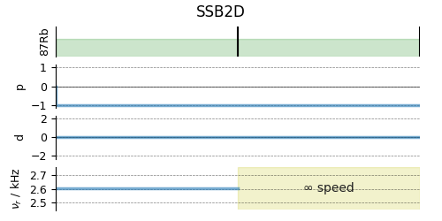
qmat = SSB2D(
    channels=["87Rb"],
    magnetic_flux_density=9.4,
    rotor_frequency=2604,
    spectral_dimensions=[
        SpectralDimension(
            count=32 * 4,
            spectral_width=2604 * 32,  # in Hz
            label="Anisotropic dimension",
        ),
        SpectralDimension(
            count=512,
            spectral_width=50000,  # in Hz
            label="Fast MAS dimension",
        ),
    ],
)

# A graphical representation of the method object.
plt.figure(figsize=(5, 2.5))
qmat.plot()
plt.show()

Create the Simulator object, add the method and spin system objects, and run the simulation.

sim = Simulator(spin_systems=spin_systems, methods=[qmat])

# For 2D spinning sideband simulation, set the number of spinning sidebands in the
# Simulator.config object to `spectral_width/rotor_frequency` along the sideband
# dimension.
sim.config.number_of_sidebands = 32
sim.run()

The plot of the simulation.

plt.figure(figsize=(4.25, 3.0))
dataset = sim.methods[0].simulation.real
ax = plt.subplot(projection="csdm")
cb = ax.imshow(dataset / dataset.max(), aspect="auto", cmap="gist_ncar_r", vmax=0.15)
plt.colorbar(cb)
ax.invert_xaxis()
ax.set_ylim(200, -200)
plt.tight_layout()
plt.show()

1

Walder, B. J., Dey, K .K, Kaseman, D. C., Baltisberger, J. H., and Philip J. Grandinetti. Sideband separation experiments in NMR with phase incremented echo train acquisition, J. Chem. Phys. (2013) 138, 174203. DOI:10.1063/1.4803142