Wollastonite, ²⁹Si (I=1/2), MAF¶

²⁹Si (I=1/2) magic angle flipping.

Wollastonite is a high-temperature calcium-silicate, \(\beta−\text{Ca}_3\text{Si}_3\text{O}_9\), with three distinct \(^{29}\text{Si}\) sites. The \(^{29}\text{Si}\) tensor parameters were obtained from Hansen et al. [1]

import numpy as np
import matplotlib.pyplot as plt

from mrsimulator import Simulator, SpinSystem, Site
from mrsimulator import signal_processor as sp
from mrsimulator.spin_system.tensors import SymmetricTensor
from mrsimulator.method import Method, SpectralDimension, SpectralEvent, MixingEvent

Create the sites and spin systems

sites = [
    Site(
        isotope="29Si",
        isotropic_chemical_shift=-89.0,  # in ppm
        shielding_symmetric=SymmetricTensor(zeta=59.8, eta=0.62),  # zeta in ppm
    ),
    Site(
        isotope="29Si",
        isotropic_chemical_shift=-89.5,  # in ppm
        shielding_symmetric=SymmetricTensor(zeta=52.1, eta=0.68),  # zeta in ppm
    ),
    Site(
        isotope="29Si",
        isotropic_chemical_shift=-87.8,  # in ppm
        shielding_symmetric=SymmetricTensor(zeta=69.4, eta=0.60),  # zeta in ppm
    ),
]

spin_systems = [SpinSystem(sites=[s]) for s in sites]

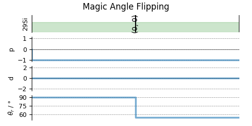
Use the generic Method class to simulate a 2D magic-angle Flipping (MAF) spectrum by customizing the method parameters, as shown below.

Here, we include a MixingEvent with a NoMixing query. A no mixing query instructs the MAF method to not mix the transitions from the first and second SpectralEvent. A no mixing query is equivalent to a rotation query where each channel has a zero phase and angle. Since all spin systems in this example have a single site, defining no mixing between the two spectral events is superfluous. We include it such that the method is applicable with multi-site spin systems.

maf = Method(
    name="Magic Angle Flipping",
    channels=["29Si"],
    magnetic_flux_density=14.1,  # in T
    rotor_frequency=np.inf,
    spectral_dimensions=[
        SpectralDimension(
            count=128,
            spectral_width=2e4,  # in Hz
            label="Anisotropic dimension",
            events=[
                SpectralEvent(
                    rotor_angle=90 * np.pi / 180,  # in rads
                    transition_queries=[{"ch1": {"P": [-1], "D": [0]}}],
                ),
                MixingEvent(query="NoMixing"),
            ],
        ),
        SpectralDimension(
            count=128,
            spectral_width=3e3,  # in Hz
            reference_offset=-1.05e4,  # in Hz
            label="Isotropic dimension",
            events=[
                SpectralEvent(
                    rotor_angle=54.735 * np.pi / 180,  # in rads
                    transition_queries=[{"ch1": {"P": [-1], "D": [0]}}],
                )
            ],
        ),
    ],
    affine_matrix=[[1, -1], [0, 1]],
)

# A graphical representation of the method object.
plt.figure(figsize=(5, 2.5))
maf.plot()
plt.show()

Create the Simulator object, add the method and spin system objects, and run the simulation.

sim = Simulator(spin_systems=spin_systems, methods=[maf])
sim.run()

Add post-simulation signal processing.

csdm_dataset = sim.methods[0].simulation
processor = sp.SignalProcessor(
    operations=[
        sp.IFFT(dim_index=(0, 1)),
        sp.apodization.Gaussian(FWHM="50 Hz", dim_index=0),
        sp.apodization.Gaussian(FWHM="50 Hz", dim_index=1),
        sp.FFT(dim_index=(0, 1)),
    ]
)
processed_dataset = processor.apply_operations(dataset=csdm_dataset).real
processed_dataset /= processed_dataset.max()

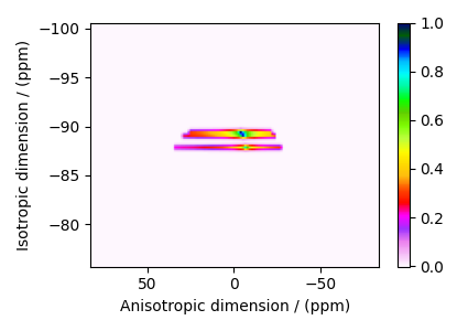
The plot of the simulation after signal processing.

plt.figure(figsize=(4.25, 3.0))
ax = plt.subplot(projection="csdm")
cb = ax.imshow(processed_dataset.T, aspect="auto", cmap="gist_ncar_r")
plt.colorbar(cb)
ax.invert_xaxis()
ax.invert_yaxis()
plt.tight_layout()
plt.show()

Total running time of the script: (0 minutes 0.648 seconds)

Gallery generated by Sphinx-Gallery